METROPOLIS2 Course
Session 1
Lucas Javaudin
2025
Plan of this Session
- Overview of METROPOLIS2
- A bit of theory
- METROPOLIS2 Getting Started
-
"Manual" simulation generation
- Supply side
- Demand side
- Run
- Output analysis
Plan of this Session
- Overview of METROPOLIS2
- A bit of theory
- METROPOLIS2 Getting Started
-
"Manual" simulation generation
- Supply side
- Demand side
- Run
- Output analysis
A Bit of History
- 1997-2009: Simulator METROPOLIS1 [C++] (de Palma, Marchal, Nesterov)
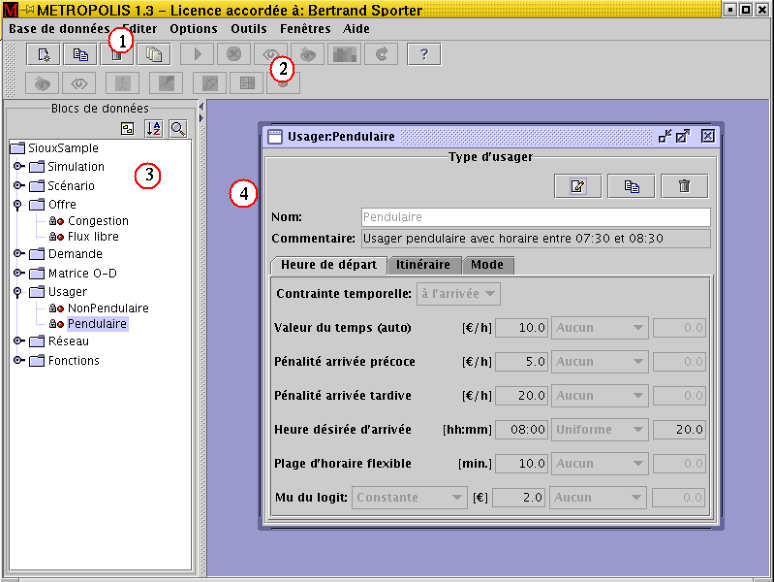
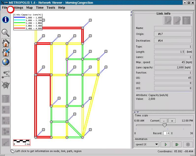
- 2001-2009: Interface for METROPOLIS1 [Java] (Marchal)
- 2018-2021: Web interface for METROPOLIS1 [Python Django] (Javaudin)
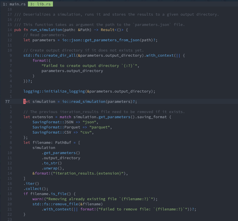
- 2021-: METROPOLIS2 [Rust] (de Palma, Javaudin)

What is METROPOLIS2
Transport simulator with the following characteristics:
- Simulate mode, departure-time and route choice
- Agent-based
- Multi-modal
- Micro-founded
- Dynamic
- Adapted for small- and large-scale simulations
- Fast
- Extensible
General Flow
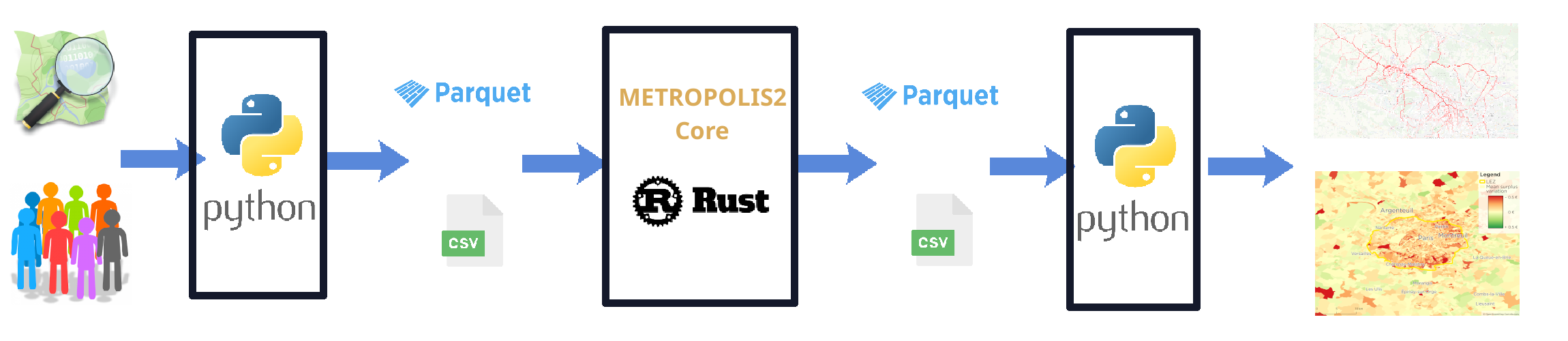
- Python scripts are used to convert data to the simulator's input files
- The METROPOLIS2 simulator reads the input files and writes output files (Parquet or CSV format)
- Python scripts are used to read the output files and produce results
Python scripts can be shared between users or replaced by other tools
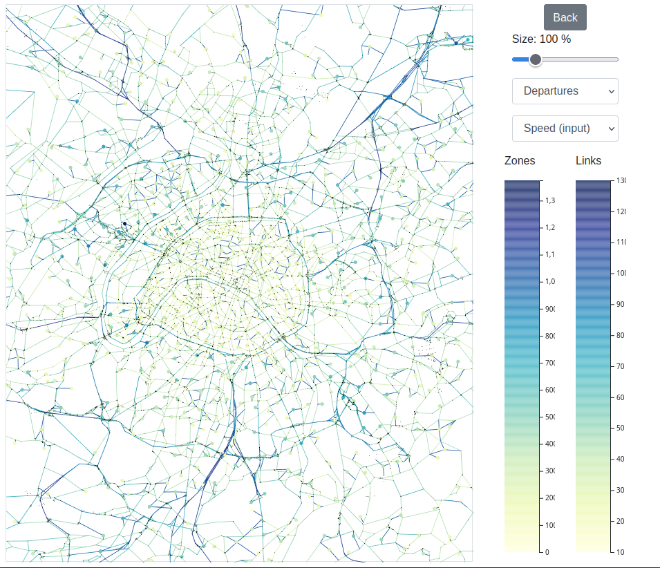
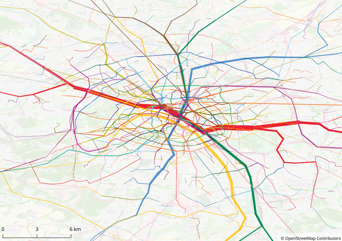
Examples of Productions
Public-transit flows by line, Paris' urban area, Morning peak
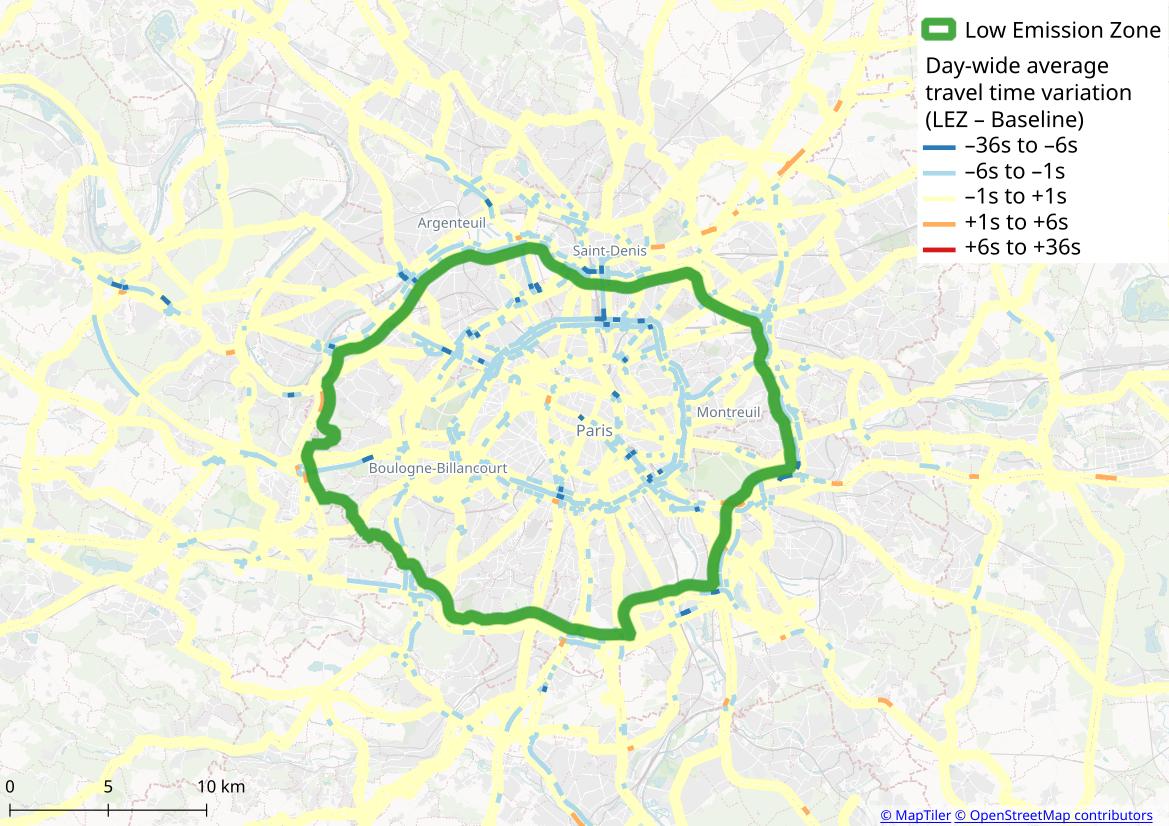
Road-level congestion variation when Paris' Low Emission Zone is implemented
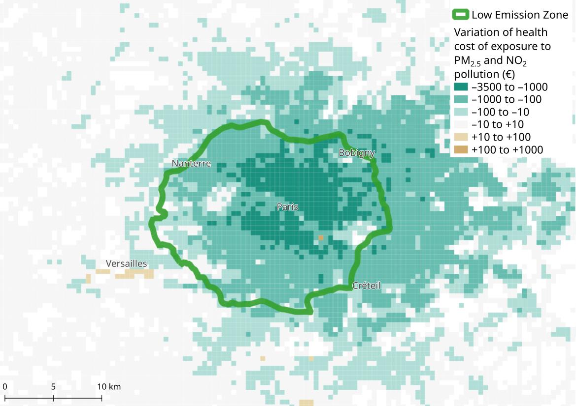
Variation of exposure cost to air pollution when Paris' Low Emission Zone is implemented
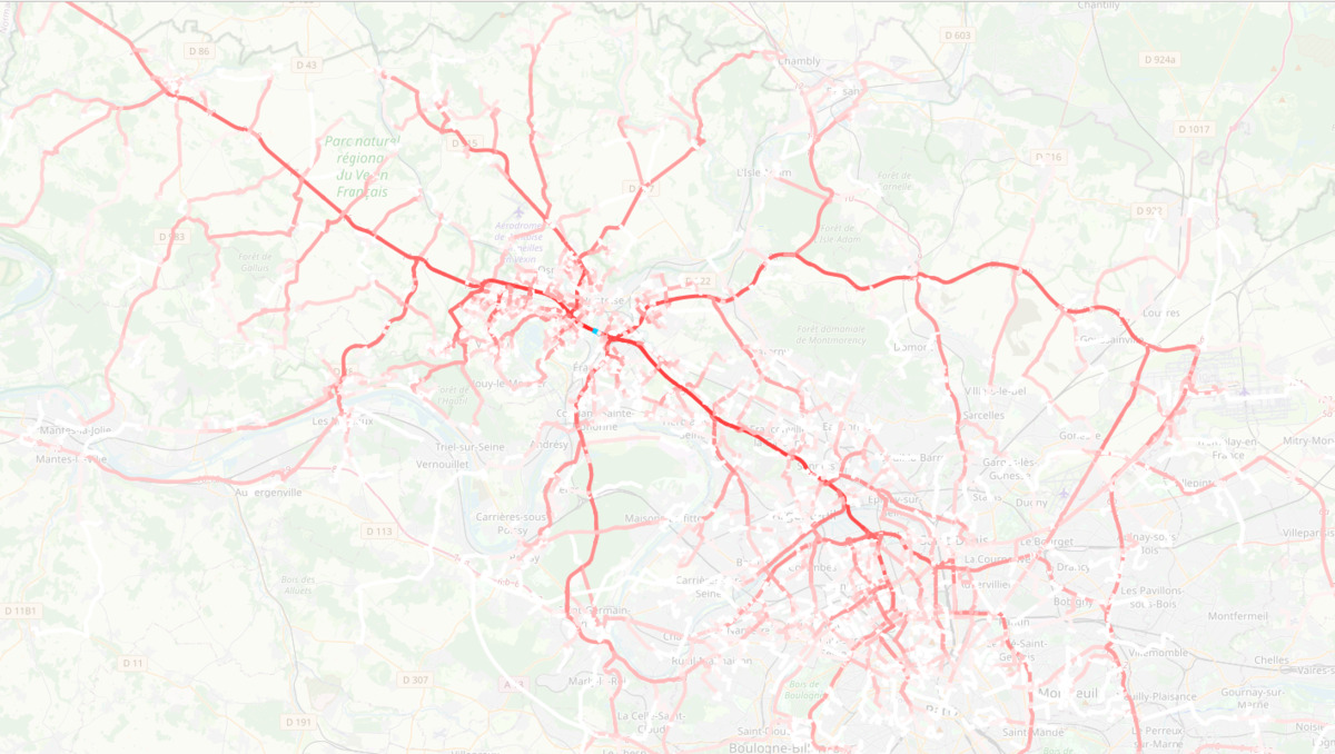
Car flows for all trips going through highway A15 near Cergy
Vehicle movements in the surroundings of Cergy, 08:00 to 08:05
Plan of this Session
- Overview of METROPOLIS2
- A bit of theory
- METROPOLIS2 Getting Started
-
"Manual" simulation generation
- Supply side
- Demand side
- Run
- Output analysis
The Bottleneck Model
-
A road is connecting an origin $A$ to a destination $B$: free-flow travel time is $t^f$ and there is a point-bottleneck of capacity $s$
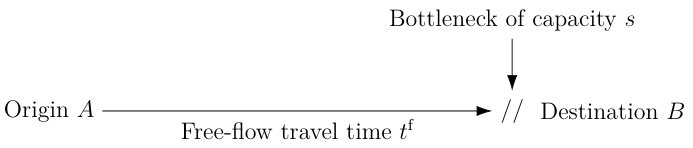
- Travel time from $A$ to $B$ is \[ t^f + \frac{Q(t + t^f)}{s} \] with $Q$ the length of the bottleneck queue at time $t$.
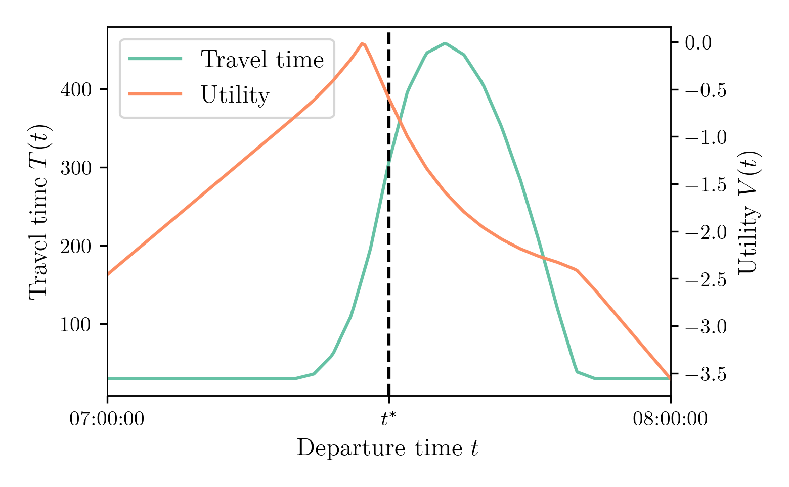
Alpha-Beta-Gamma Utility
Utility is given by \[ V(t) = -\alpha \cdot T(t) - \beta \cdot [t^* - t - T(t)]_+ - \gamma \cdot [t + T(t) - t^*]_+ \]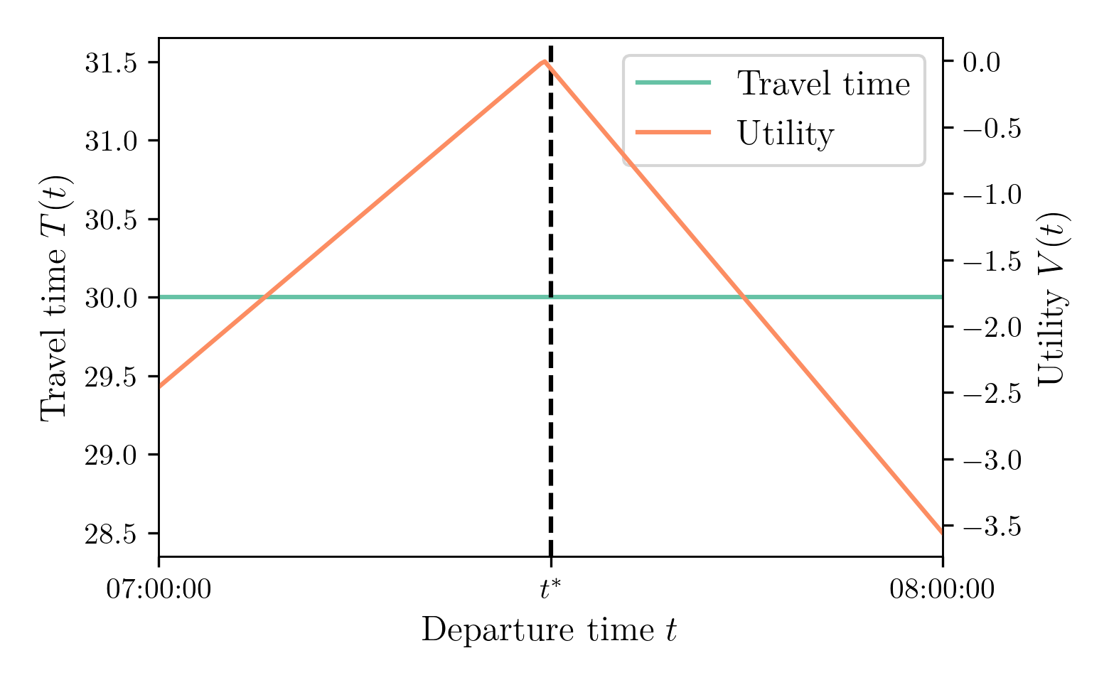
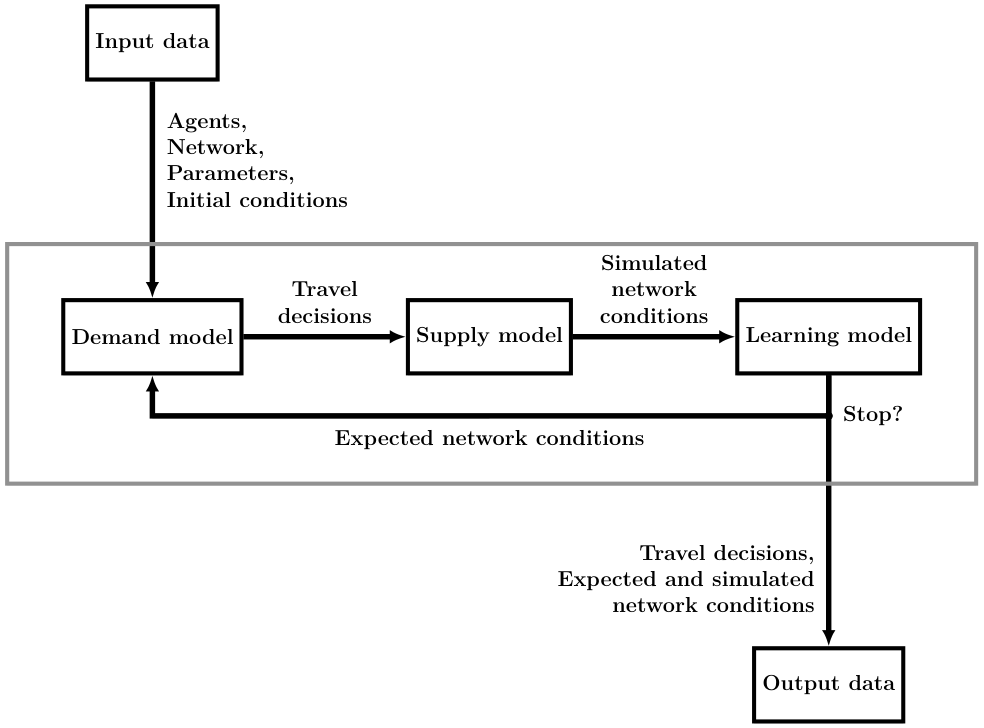
METROPOLIS2 Fundamental Flow Diagram
Plan of this Session
- Overview of METROPOLIS2
- A bit of theory
- METROPOLIS2 Getting Started
-
"Manual" simulation generation
- Supply side
- Demand side
- Run
- Output analysis
Files Format: JSON
-
Collection of key-value pairs that can be nested indefinitely
{ "key": "value", "integer": 1, "float": 3.6, "boolean": true, "array": [ 0, 1, 2 ], "nested_array": [ {"some": "value"}, {"another": "value"} ] } - Very close to Python's
dicttype - Format used to configure the parameters of a METROPOLIS2 simulation and for some output files
- Syntax definition: https://en.wikipedia.org/wiki/JSON#Syntax
Files Format: CSV
- Row-oriented file format for tabular data
- Human readable
- Compatible with many tools and languages (including Excel!)
- Used in METROPOLIS2 for most input and output files (comma separator only)
- Recommended only for small-scale simulations, especially when using Excel
						col1,col2,col3,col4
						1,Alice,3.2,true
						2,Bob,1.4,false
						3,Charlie,2.5,false
Files Format: Parquet
- Column-oriented file format for tabular data
- Binary file (= non human-readable)
- Built-in compression: smaller file size than CSV
- Very fast
- Compatible with Python (polars or pandas libraries) and R (arrow package)
- Used in METROPOLIS2 for most input and output files
- Recommended format for large-scale simulations and people working with R or Python
						import polars as pl

						df = pl.DataFrame(
								{
										"agent_id": [0, 1, 2],
										"alt_choice.type": ["Deterministic", "Logit", "Logit"],
										"alt_choice.u": [0.3, 0.6, 0.5],
										"alt_choice.mu": [None, 0.9, 1.0],
										"alt_choice.constants": [[0.9, 1.3, 2.1], None, None],
								}
						)
						df.write_parquet("input/agents.parquet")
						In [3]: df
						Out[3]:
						shape: (3, 5)
						┌──────────┬─────────────────┬──────────────┬───────────────┬──────────────────────┐
						│ agent_id ┆ alt_choice.type ┆ alt_choice.u ┆ alt_choice.mu ┆ alt_choice.constants │
						│ ---      ┆ ---             ┆ ---          ┆ ---           ┆ ---                  │
						│ i64      ┆ str             ┆ f64          ┆ f64           ┆ list[f64]            │
						╞══════════╪═════════════════╪══════════════╪═══════════════╪══════════════════════╡
						│ 0        ┆ Deterministic   ┆ 0.3          ┆ null          ┆ [0.9, 1.3, 2.1]      │
						│ 1        ┆ Logit           ┆ 0.6          ┆ 0.9           ┆ null                 │
						│ 2        ┆ Logit           ┆ 0.5          ┆ 1.0           ┆ null                 │
						└──────────┴─────────────────┴──────────────┴───────────────┴──────────────────────┘
METROPOLIS2 Input Files
- Parameters (JSON)
-
Supply side:
- Road network (Parquet or CSV)
- Vehicle types (Parquet or CSV)
-
Demand side:
- Agents (Parquet or CSV)
- Travel alternatives (Parquet or CSV)
- Trips (Parquet or CSV)
- Optional road-network conditions (Parquet or CSV)
METROPOLIS2 Output Files
- HTML summary
- Aggregated results by iteration (Parquet or CSV)
-
Supply side:
- Link-level time-dependent travel times (simulated, expected for last iteration and expected for next iteration) (Parquet or CSV)
- OD-level time-dependent travel times (expected for last iteration) (JSON, for now)
-
Demand side:
- Agent-level results (Parquet or CSV)
- Trip-level results (Parquet or CSV)
- Routes taken (Parquet or CSV)
Units
For consistency and to prevent mistakes, METROPOLIS2 uses the same units for all input and output variables.
| Type | Unit | Example |
|---|---|---|
| Time of day | Seconds after midnight | 8 * 3600 = 28800 is 8 a.m. |
| Time duration | Seconds | 300 (5 minutes) |
| Length | Meters | |
| Speed | Meters / Second | 50 / 3.6 = 13.89 m/s is 50 km/h |
| Passenger Car Equivalent (PCE) | N/A | Usually normalized to 1 for car |
| Flow | PCE / Second | 0.5 PCE/s = 1800 PCE per hour |
| Utility | No specific unit (can be monetary units) | |
| Value of Time | Utility / Second | 15 / 3600 = 0.004167 is 15 $/h |
Mistakes are still possibles, be careful!
Documentation
The documentation (WIP) is the best way to understand the input and output formats
https://docs.metropolis.lucasjavaudin.comRunning METROPOLIS2
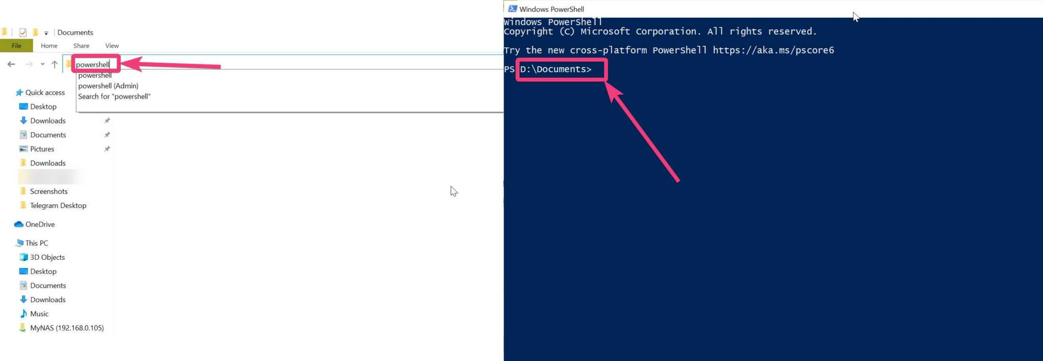
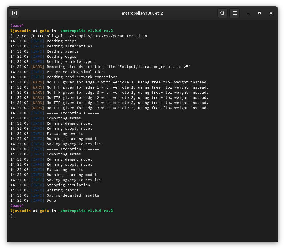
- Open a Command prompt / Terminal / Powershell with the working directory set to the location of the unzipped directory
-
For Windows, run:
.\execs\metropolis_cli.exe .\examples\data\csv\parameters.json -
For MacOS or Linux, run:
./execs/metropolis_cli ./examples/data/csv/parameters.json - Check that the run succeeded
- The results are stored in
examples/data/csv/output/
Plan of this Session
- Overview of METROPOLIS2
- A bit of theory
- METROPOLIS2 Getting Started
-
"Manual" simulation generation
- Supply side
- Demand side
- Run
- Output analysis
Sources of Congestion
- Bottleneck: the inflow and outflow of vehicles is limited at the link-level
- Speed-density function: the speed of vehicles depends on the density of vehicles currently on the link
- Queue propagation (or spillback, or horizontal queues): vehicles can enter a link only if there is some space available
Vehicle Types
- Headway length (head-to-head) → for speed-density functions and spillback evaluation
- PCE (Passenger Car Equivalent) → for bottlenecks
- Speed functions → e.g., to represent speed limits
- Road restrictions → allowed / forbidden links
Simplified Process
- Cross the entry bottleneck if it is open, or wait until it opens
- Enter the link if there is some space available, or wait for some space to be available again
- Travel across the length of the link at a constant speed given based on the density of vehicles on the link at the entry time
- Cross the exit bottleneck if it is open, or wait until it opens
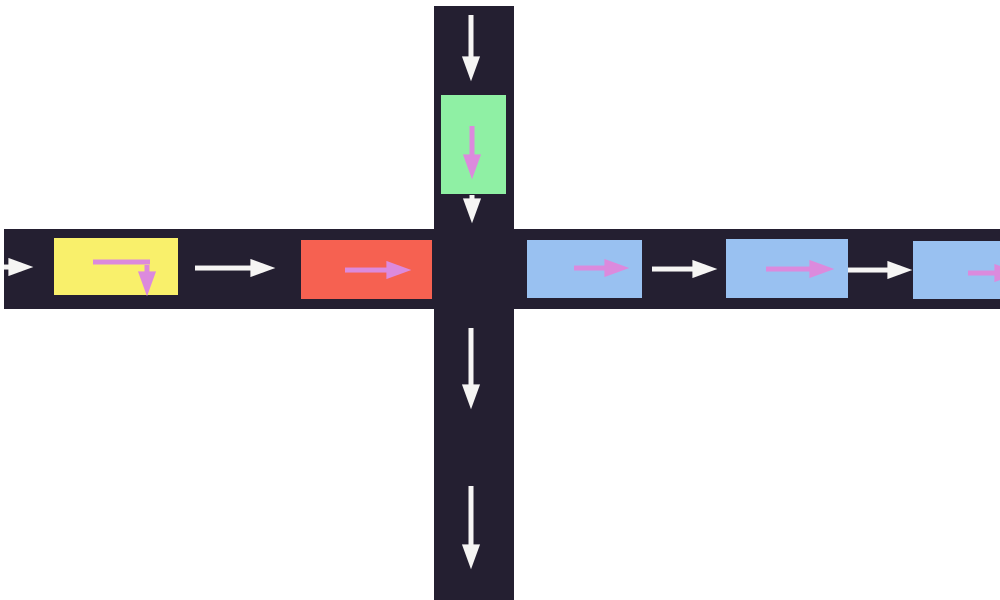
Bottleneck
- One bottleneck at the entry and exit of each link
- Bottlenecks can be in two states: open or closed
- Bottlenecks are open by default and open bottlenecks can be crossed immediately
- When a vehicle cross a bottleneck, the bottleneck gets closed for a duration \[ \text{closing time} = \frac{\text{Vehicle PCE}}{\text{Bottleneck flow}} \]
- When a vehicle reaches a closed bottleneck, it is pushed to the back of the bottleneck queue
- When a closed bottleneck re-opens, the vehicle at the front of the queue can cross
- Question: bottleneck flow of 1200 PCE/h; a truck (3 PCEs) is crossing it; what is the closing time?
- Answer: 3 / (1/3) = 9
Overtaking
- When traveling to the end of the link, faster moving vehicles can overtake slower vehicles
- By default, when a vehicle is stuck at the entry of a link (entry bottleneck closed or no space available), the exit bottleneck of the previous link stays closed → vehicles upstream are also stuck
- If enabled, the exit bottleneck of the previous link re-opens as soon as a vehicle cross (even if it is stuck downstream) → vehicles upstream can overtake the vehicle if they are going to different downstream links
Number of Lanes
- The bottleneck flow of a link is multiplied by the number of lanes
- The space available on the link is multiplied by the number of lanes (relevant for spillback only)
Speed-Density Functions
- The speed at which a vehicle travel over the length of an edge is constant and computed using the edge's speed-density function
- The speed-density returns the traveling speed on the edge as a function of the current density of vehicles on the edge
- The edge's density is computed as \[ \text{density} = \frac{\sum_{\text{vehicle on the edge}}\text{headway length of vehicle}}{\text{length} \times \text{lanes}} \]
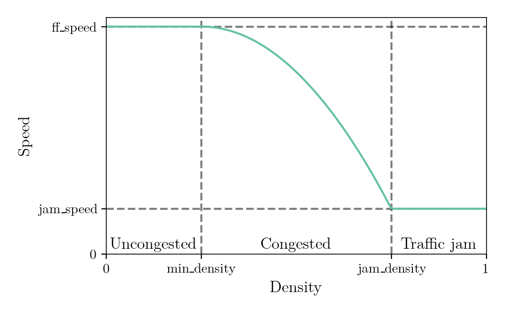
- Three speed-density functions: FreeFlow (default), Bottleneck (METROPOLIS1 legacy), ThreeRegimes
Speed-Density Functions: Three Regimes
Spillback
- If spillback is enabled, vehicles can enter an edge only if there some room left on the edge ($\Leftrightarrow$ density < 1)
- If the edge ahead is full, the vehicle is remaining in the exit bottleneck queue of the current edge, in a "pending state"
- When a vehicle exits an edge, the space taken by this vehicle propagates backward at a given speed (backward wave propagation)
- Time at which the space of an outgoing vehicle is made available for the incoming vehicles: \[ \text{exit\_time} + \frac{\text{length}}{\text{backward\_wave\_speed}} \]
Gridlocks
- When spillback is enabled, the road network can reach a state where some vehicles are permanently stuck
- The maximum pending duration defines the maximum amount of time a vehicle can be in a pending state
- After the maximum pending duration elapses, pending vehicles are forced onto the next edge
Overview
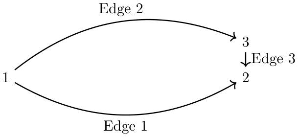
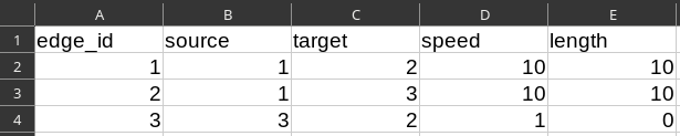
- The simulator represents the road network as a directed graph of nodes (= intersections) and edges (= links)
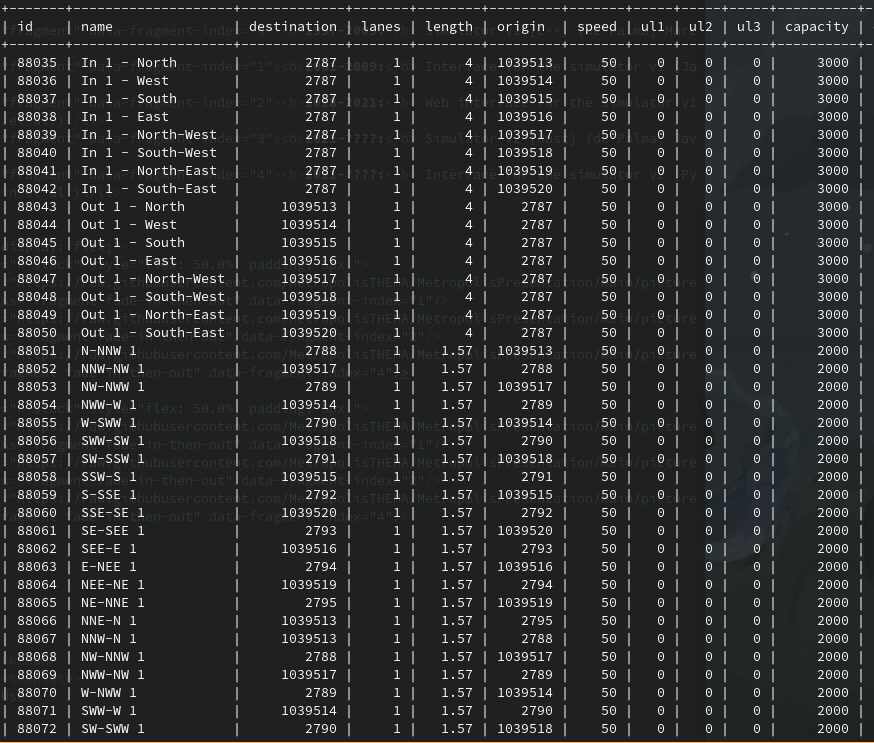
- METROPOLIS2 takes as input a list of edges
Edges: Minimal Example
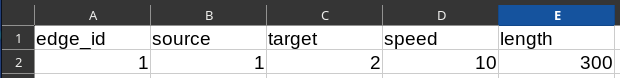
edge_id: Identifier of the edge (positive integer, unique)source: Identifier of the source node (positive integer)target: Identifier of the target node (positive integer)speed: Free-flow speed on the edge (m/s)length: Length of the edge (m)
Bottleneck

bottleneck_flow: Maximum inflow and outflow of the edge (PCE/s)- When the variable is omitted, the inflow and outflow are not limited
Bottleneck Overtaking
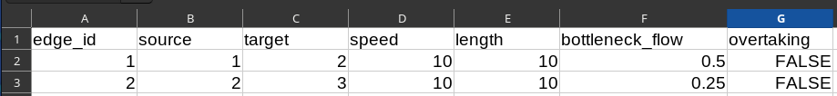
overtaking: If `True`, vehicles can overtake other vehicles in the bottleneck queues if they are going to different edges- Default value is `True`
Number of Lanes

lanes: number of lanes available to vehicles on the edge (in the current direction)- If omitted, the number of lanes is set to 1
- Non-integer values can be used
Travel Time Penalty

constant_travel_time: time penalty that is added to the edge's travel time, in seconds- Travel-time on the edge is (excluding the waiting times): \[ \text{constant\_travel\_time} + \frac{\text{length}}{\text{speed}(\text{density})} \]
- This penalty can represent delays which happen even under free-flow conditions (e.g., waiting at traffic lights, stopping at a stop sign)
- The default value is zero
Parallel Edges
-
The METROPOLIS2 Routing algorithm cannot handle edges with the same source and target (parallel edges)
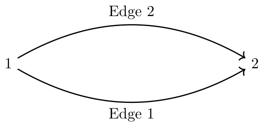
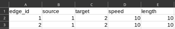
-
Possible workaround if required:
Vehicle Types: Minimal Example
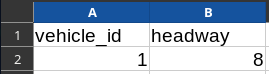
vehicle_id: Identifier of the vehicle (positive integer, unique)headway: Head-to-head length between two vehicles (m, used to compute edge's density)
Passenger-Car Equivalent
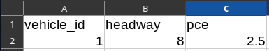
pce: Passenger-car equivalent for the vehicle (non-negative number)- Used to compute the closing time of bottlenecks
- Default value is 1
Speed Function
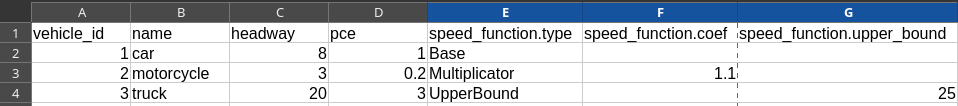
- The "Multiplicator" speed function type can be used to increase / decrease the speed of vehicles by a multiplicative coefficient
- The "UpperBound" speed function type can be used to specify a maximum speed that the vehicles cannot exceed (e.g., trucks limited to 90 km/h)
Road Restrictions

- Cars are allowed on all edges
- Motorcycles are only allowed on edges 1 and 2
- Trucks are allowed on all edges but edges 3 and 4
- Warning: lists are only supported for the Parquet format so the road restrictions do not work for CSV
Road Network Parameters
- The parameters JSON input file contains configuration values for the simulation (e.g., path to the input files, simulated period, learning model)
- A part of the file is dedicated to road-network parameters
- The remaining parts will be covered in the next sections
							{
								[...]
								"road_network": {
									"recording_interval": 300.0,
									"approximation_bound": 1.0,
									"spillback": true,
									"backward_wave_speed": 4.0,
									"max_pending_duration": 60.0,
									"constrain_inflow": true,
									"algorithm_type": "Best",
								},
								[...]
							}
Travel-Time Function Parameters
recording_interval: time, in seconds, between two breakpoints in the edge-level travel-time functions (Mandatory; Recommendation: 5, 10 or 15 minutes for large-scale networks)approximation_bound: for a given travel-time function, if the difference between the maximum and the minimum travel time is smaller than this value, the function is represented as a constant function for optimization (Default: 0; Recommendation: between 0 and 5 seconds)
							{
								[...]
								"road_network": {
									"recording_interval": 300.0,
									"approximation_bound": 1.0,
									"spillback": true,
									"backward_wave_speed": 4.0,
									"max_pending_duration": 60.0,
									"constrain_inflow": true,
									"algorithm_type": "Best",
								},
								[...]
							}
Spillback Parameters
spillback: whether spillback congestion (queue propagation) is enabled (Default: TRUE; Recommendation: TRUE for more realistic congestion modeling)backward_wave_speed: speed at which the space taken by vehicles propagates backward upon exit (Default: instantaneous propagation; Recommendation: default or 15 km/h = 4.17 m/s)max_pending_duration: maximum amount of time a vehicle can stay in a pending state (Mandatory; Recommendation: between 30s and 5m, larger values are more realistic but generate more congestion)
							{
								[...]
								"road_network": {
									"recording_interval": 300.0,
									"approximation_bound": 1.0,
									"spillback": true,
									"backward_wave_speed": 4.0,
									"max_pending_duration": 60.0,
									"constrain_inflow": true,
									"algorithm_type": "Best",
								},
								[...]
							}
Other Parameters
constrain_inflow: whether bottlenecks limit vehicle inflow in addition to vehicle outflow (Default: TRUE; Recommendation: TRUE, set to FALSE to replicate MATSim behavior)algorithm_type: routing algorithm to use for profile queries, "Best", "TCH", or "Intersect" (Default: "Best"; Recommendation: "Intersect" for a smaller running time, "TCH" for a smaller memory consumption)
							{
								[...]
								"road_network": {
									"recording_interval": 300.0,
									"approximation_bound": 1.0,
									"spillback": true,
									"backward_wave_speed": 4.0,
									"max_pending_duration": 60.0,
									"constrain_inflow": true,
									"algorithm_type": "Best",
								},
								[...]
							}
Plan of this Session
- Overview of METROPOLIS2
- A bit of theory
- METROPOLIS2 Getting Started
-
"Manual" simulation generation
- Supply side
- Demand side
- Run
- Output analysis
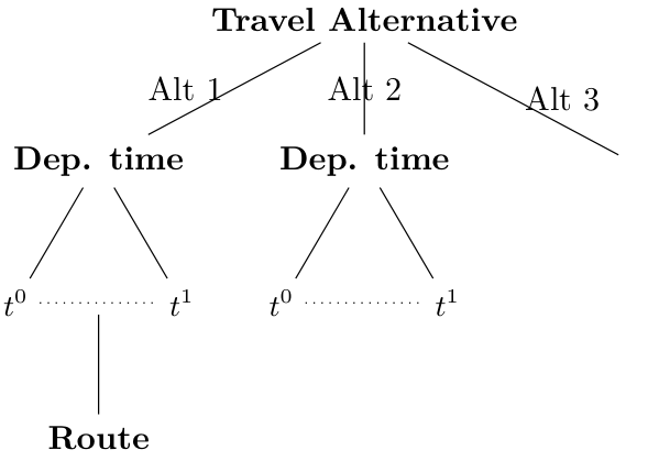
METROPOLIS2 Decision Tree
- Level 1: choice between travel alternatives
- Level 2: choice of a departure time (except for no-trip alternatives)
- Level 3: choice of a route (for road trips only)
Travel Alternatives
- Travel alternative: description of a plan / program / strategy that the agent can choose to execute
- Examples: travel from home to work by car; travel from home to work by public-transit then from work to shop by walking; do not travel
- All agents must have at least one alternative
- At each iteration, each agent is selecting exactly one alternative to execute
- In most cases, the choice of an alternative represents a mode choice
Logit Model
- Consider an agent choosing between two alternatives 1 and 2
- (Deterministic) utility of alternative 1 (resp. 2) is $V_1$ (resp. $V_2$)
- Discrete-choice theory: total utility of alternative $j$ is \[ U_j = V_j + \varepsilon_j \]
- Logit model if $\varepsilon_j \overset{i.i.d.}{\sim} \textit{Gumbel}$
- Probability to choose alternative $1$ is \[ p_1 = \text{Prob}(U_1 > U_2) = \frac{e^{V_1}}{e^{V_1} + e^{V_2}} \]
- Expected utility from the choice \[ \mathbb{E}_{\varepsilon}[\max_j U_j] = \ln(e^{V_1} + e^{V_2}) + 0.577 \]
Multinomial Logit and Continuous Logit
- Probability to choose alternative $j$: \[ p_j = \frac{e^{V_j / \mu}}{\sum_k e^{V_k / \mu}} \]
- Expected utility from the choice \[ \mathbb{E}_{\varepsilon}[\max_j U_j] = \mu \ln \sum_j e^{V_j / \mu} + \mu \cdot 0.577 \]
- Probability to choose interval $[t, t']$: \[ p([t, t']) = \frac{\int_{t}^{t'} e^{V(\tau) / \mu} \text{d} \tau}{\int_{t^0}^{t^1} e^{V(\tau) / \mu} \text{d} \tau} \]
- Expected utility from the choice \[ \mathbb{E}_{\varepsilon}[\max_\tau U(\tau)] = \mu \ln \int_{t^0}^{t^1} e^{V(\tau) / \mu} \text{d} \tau + \mu \cdot 0.577 \]
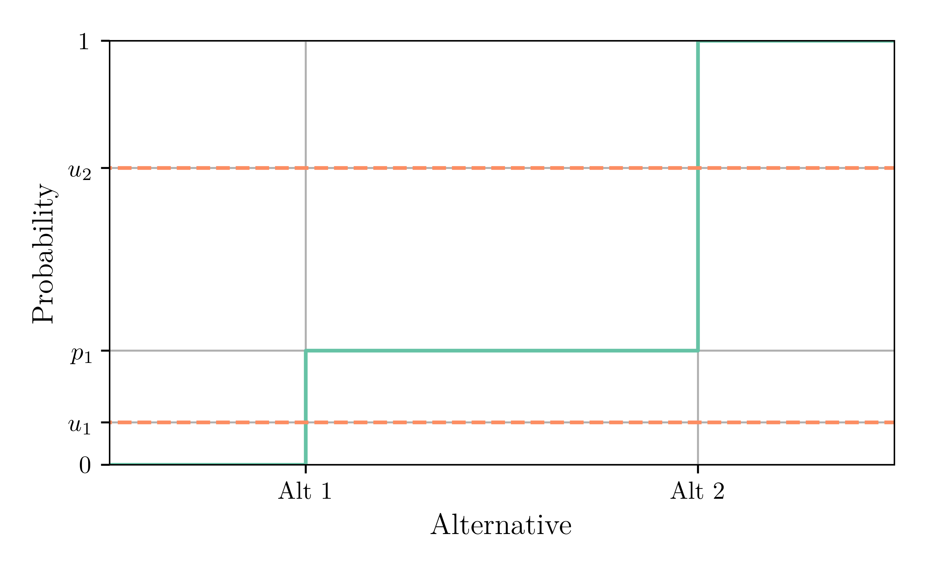
Inverse Transform Sampling
- Draw a value $u_n \sim \text{Uniform}([0, 1])$ for each agent
- Select alternative 1 if $u_n < p_1$
Trips
- Each alternative consists in 0, 1 or more trip(s), to be executed sequentially
- Two types of trips: road and virtual
- Road trip: origin, destination, vehicle type
- Virtual trip (or teleport trip): exogenous travel time (e.g., walking, cycling, public transit)
Trip Chaining
- Each alternative can contain an arbitrary number of trips (a mix of road and virtual trips is possible)
- The trips are performed in the order in which they appear in the trips input file
- The
stopping_timevariable can be used to add a delay between two trips (this can represent the activity duration)
Departure-Time Choice
- Three types of departure-time approaches: Constant (dynamic traffic assignment), Continuous choice (Continuous Logit model), Discrete choice
- The only decision variable for departure-time choice is the departure time for the first trip of the trip chain → the departure time for the subsequent trips depends of the previous' trips travel times and stopping times
- The departure-time choice is based on the (anticipated) utility for the entire trip chain
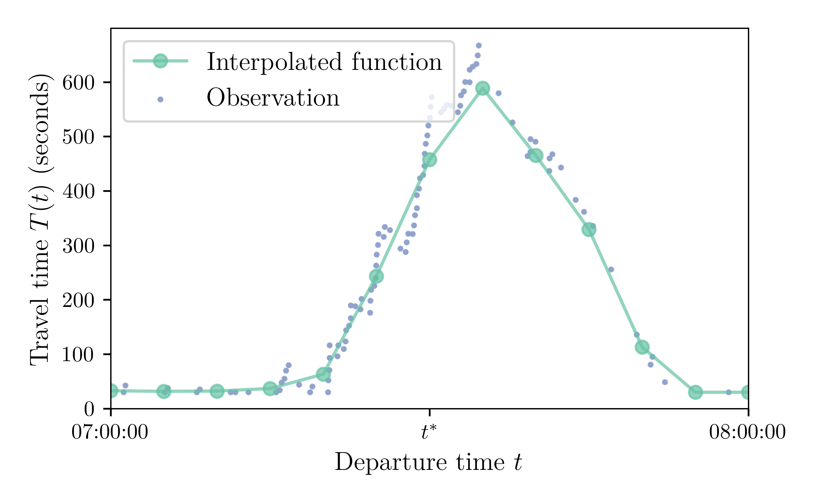
Continuous Logit
- Probability to choose interval $[t, t']$: \[ p([t, t']) = \frac{\int_{t}^{t'} e^{V(\tau) / \mu} \text{d} \tau}{\int_{t^0}^{t^1} e^{V(\tau) / \mu} \text{d} \tau} \]
- Expected utility from the choice \[ \mathbb{E}_{\varepsilon}[\max_\tau U(\tau)] = \mu \ln \int_{t^0}^{t^1} e^{V(\tau) / \mu} \text{d} \tau + \mu \cdot 0.577 \]
- Probability to choose interval $[t, t']$: \[ p([t, t']) = \frac{t' - t}{t^1 - t^0} \]
- Expected utility from the choice \[ \mathbb{E}_{\varepsilon}[\max_\tau U(\tau)] = \bar{V} + \mu \cdot \ln(t^1 - t^0) + \mu \cdot 0.577 \]
Utility
- Utility of a trip is \[ \text{trip utility} = \text{travel utility} + \text{schedule utility} \] with \[ \text{travel utility} = \texttt{travel\_utility.one} \times {tt} \] and \[ \text{schedule utility} = -\texttt{beta} \times [\texttt{tstar} - t^a]_+ - \texttt{gamma} \times [t^a - \texttt{tstar}]_+ \]
- Total utility of a travel alternative is \[ \text{utility} = \texttt{constant\_utility} + \sum_{\text{trip}} \text{trip utility} \]
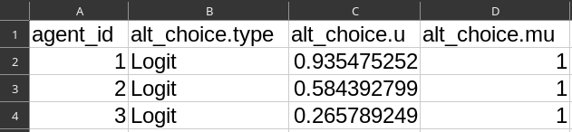
Agents input file
File agents.csv
Define agents and their choice model between alternatives
Alternatives input file
File alts.csv:
Define alternatives for each agent, with the constant utility and departure-time choice model (except for alternatives with no trip)

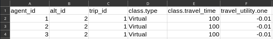
Trips input file
File trips.csv:
Define the trips of each alternative, with the type (road / virtual), characteristics (origin, destination, travel time), and travel and schedule utility parameters
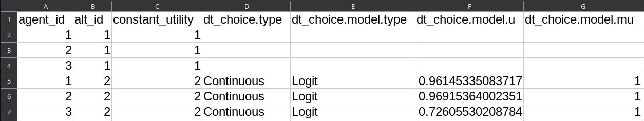
Continuous Departure-Time Choice Example
File alts.csv:
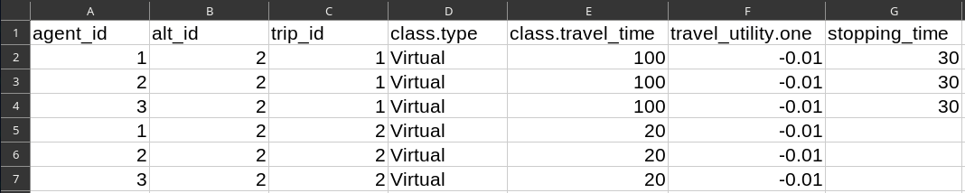
Trip Chaining Example
File trips.csv:
stopping_time is the time that elapses before the next trip starts
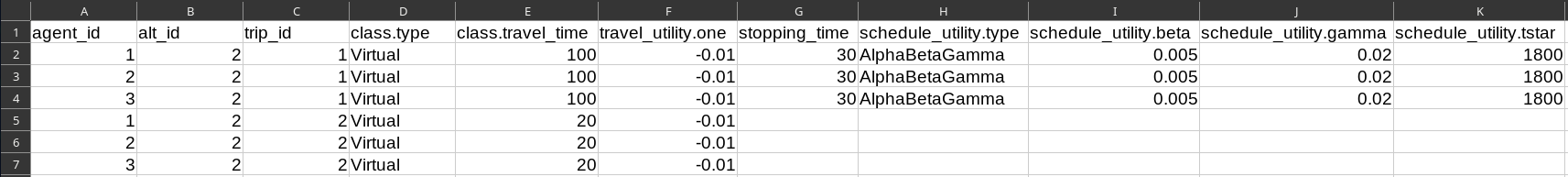
Schedule-Delay Utility Example
File trips.csv:
Warning: travel_utility.one is expressed in utility / second; schedule_utility.beta and schedule_utility.gamma are expressed in "generalized cost" / second
Alternative Choice
- At the top level, agents choose among an arbitrary number of travel alternatives
- A travel alternative is defined as a sequence of trips and a utility function specification
-
The alternative choice can represent:
- Mode choice: H→W by car | H→W by PT | H→W by walk
- Mode choice with trip chaining: H→W→S→H by car | H→W→S→H by bicycle
- To travel or not to travel: H→W by car | No trip (work-from-home)
- Inter-modality: H→P by car then P→W by PT | H→W by car
- Destination choice: H→S1 by walk | H→S2 by walk
- Vehicle choice: H→W with a fast but energy-consuming car | H→W with a fuel-efficient but slow car
Choice Models
- Alternative choice: Multinomial Logit or Deterministic
- Departure-time choice: Continuous Logit or Multinomial Logit
- Almost any discrete-choice model is feasible by drawing the epsilon values (idiosyncratic chocs) "offline" and specifying them in the utility
- Selecting alternative $A$ with probability $p = e^{V_a} / (e^{V_a} + e^{V_b})$ using inverse transform sampling is equivalent to selecting alternative $A$ if and only if $V_A + \varepsilon_A > V_B + \varepsilon_B$ where $\varepsilon_A$ and $\varepsilon_B$ are two Gumbel-distributed values
- Example for a Probit mode choice with three alternatives:
- Draw $\varepsilon_j \sim \mathcal{N}(0, 1), j \in \{1, 2, 3\}$
- Add $\varepsilon_j$ to the utility of alternative $j$ in the simulator
- Select a deterministic choice model (the value maximizing $V_j + \varepsilon_j$ is selected)
Input data
- Origin-Destination Matrix: For any row $i$ and colomun $j$ in the matrix, generate $a_{ij}$ agents with a single trip from origin $i$ to destination $j$
-
Synthetic Population:
- Given various data (census, travel survey, etc.), the synthetic population algorithm returns a list of agents and the activities they perform
- Easily convertible to METROPOLIS2 input format
- Travel times for virtual trips can be computed using METROPOLIS2's routing algorithm (See Session 2)
- Example for France: Hörl, S. and M. Balac (2021) Synthetic population and travel demand for Paris and Île-de-France based on open and publicly available data, Transportation Research Part C
Plan of this Session
- Overview of METROPOLIS2
- A bit of theory
- METROPOLIS2 Getting Started
-
"Manual" simulation generation
- Supply side
- Demand side
- Run
- Output analysis
METROPOLIS2 Fundamental Flow Diagram
Network Conditions
- The network conditions consist in a travel-time function for each link and for each vehicle type
- The travel-time functions are represented as piecewise-linear functions with a fixed interval $\delta$ between two breakpoints
- Simulated network conditions: Network conditions observed, given some travel decisions (from the supply model).
- Expected network conditions: Network conditions anticipated by the agents when taking travel decisions (in the demand model). They are used to compute road trips' travel times.
- Both simulated and expected network conditions are common knowledge to all agents.
Learning Model
- The expected network conditions for the next iteration, $\mathbf{\hat{T}}_{\kappa+1}$, depends on the simulated network conditions, $\mathbf{T}_{\kappa}$ and the expected network conditions, $\mathbf{\hat{T}}_{\kappa}$, of the current iteration.
- At iteration $\kappa$: \[ \mathbf{\hat{T}}_{\kappa + 1} = f(\kappa, \mathbf{T}_{\kappa}, \mathbf{\hat{T}}_{\kappa}) \]
- Exponential smoothing method: \[ f(\kappa, \mathbf{T}_\kappa, \mathbf{\hat{T}}_{\kappa}) = \frac{\lambda}{\alpha_{\kappa}} \mathbf{T}_\kappa + (1 - \lambda) \frac{\alpha_{\kappa}}{\alpha_{\kappa+1}} \mathbf{\hat{T}}_{\kappa} \] with $\lambda \in [0, 1]$, the smoothing factor.
- With $\lambda = 1$: "naive" learning; with $\lambda = 0$: arithmetic mean.
- Other learning functions are available and described in the documentation.
Equilibrium
- Goal of METROPOLIS2: Find a Nash equilibrium from the input data
- Nash equilibrium: No agent can improve their utility given the travel decisions of the other agents
- Informal definition: The expected network conditions when agents took their travel decisions are equal to the simulated network conditions from these travel decisions.
- Formal definition (fixed point problem): \[ f^{\text{demand}}(f^{\text{supply}}(\bar{\mathbf{z}}; \mathbf{D}); \mathbf{D}) = \bar{\mathbf{z}} \] $\mathbf{D}$: input data; $\bar{\mathbf{z}}$: equilibrium travel decisions
Recommendations
- Run METROPOLIS2 for a fixed number of iterations, then check the distance to an equilibrium
- For exponential smoothing method: With smaller $\lambda$, convergence is slower but steadier

Indicators: Road Network Conditions
exp_road_network_cond_rmse: Difference between the expected road-network conditions and the simulated road-network conditions-
Formula:
\[
\text{RMSE}_\kappa^{T} = \sqrt{\frac{1}{R} \sum_{r} \frac{1}{t^1 - t^0} \int_{t^0}^{t^1} [T_{r, \kappa}(t) - \hat{T}_{r, \kappa}(t)]^2 \text{d} t},
\]
- $T_{r, \kappa}(t)$: simulated travel time on link $r$, at time $t$, for iteration $\kappa$
- $\hat{T}_{r, \kappa}(t)$: expected travel time on link $r$, at time $t$, for iteration $\kappa$
- $R$: number of links
- $[t^0, t^1]$: simulation period
- Interpretation: Average difference in seconds between the expected and simulated travel times, over links and time
Indicators: Departure Time Shift
alt_dep_time_rmse: Difference between the departure times of the previous and current iteration-
Formula:
\[
\text{RMSE}_\kappa^{\text{dep}} = \sqrt{\frac{1}{N} \sum_n (t^{\text{d}}_{n, \kappa} - t^{\text{d}}_{n, \kappa-1})^2},
\]
- $t^{\text{d}}_{n, \kappa}$: departure time of agent $n$, at iteration $\kappa$
- $N$: number of agents
- Interpretation: By how much agents shifted their departure time from one iteration to another, only including the agents who did not switched to another alternative
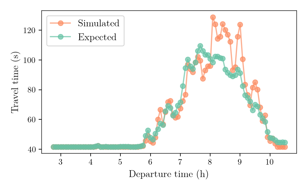
Indicators: Travel Time Expectation Error
road_trip_exp_travel_time_diff_rmse: Difference between the expected travel time and the simulated travel time-
Formula:
\[
\text{RMSE}_\kappa^{\text{expect}} = \sqrt{ \frac{1}{K^{\text{road}}} \sum_{n, k} (tt_{n, k, \kappa} - \hat{tt}_{n, k, \kappa})^2 },
\]
- ${tt}_{n, k, \kappa}$: simulated travel time for trip $k$ of agent $n$, at iteration $\kappa$
- $\hat{tt}_{n, k, \kappa}$: expected travel time for trip $k$ of agent $n$, at iteration $\kappa$
- $K^{\text{road}}$: number of road trips
- Interpretation: By how much agents mis-predicted their travel time, for their road trips
- It measures both distance to an equilibrium and approximation errors due to the linear approximation of travel-time functions
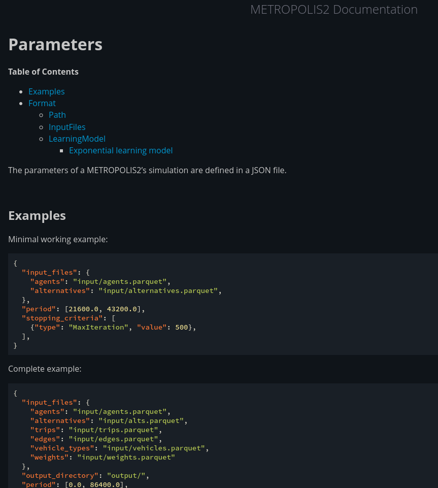
Parameters JSON File
						{
							"input_files": {
								"agents": "input/agents.parquet",
								"alternatives": "input/alts.parquet",
								"trips": "input/trips.parquet",
								"edges": "input/edges.parquet",
								"vehicle_types": "input/vehicles.parquet",
							},
							"output_directory": "output/",
							"period": [0.0, 86400.0],
							"road_network": {
									"recording_interval": 50.0,
									"approximation_bound": 1.0,
									"spillback": true,
									"backward_wave_speed": 4.0,
									"max_pending_duration": 20.0,
									"constrain_inflow": true,
									"algorithm_type": "Intersect"
							},
							"learning_model": {
								"type": "Exponential",
								"value": 0.01
							},
							"max_iterations": 20,
							"saving_format": "CSV",
						}
Plan of this Session
- Overview of METROPOLIS2
- A bit of theory
- METROPOLIS2 Getting Started
-
"Manual" simulation generation
- Supply side
- Demand side
- Run
- Output analysis
Output Files
log.txt: METROPOLIS2 log messages during the simulationrunning_times.json: simulation running time, by categoryreport.html: webpage summarizing the resultsiteration_results.{parquet,csv}: aggregate results for each iteration- 3 CSV / Parquet output files for the population results
- 4 CSV / Parquet output files for the road-network results
Running times (1/3)
File running_times.json
						{
							"total": "49181.060006808",
							"total_skims_computation": "37804.951886765",
							"total_demand_model": "2943.497363545",
							"total_supply_model": "8150.961492634",
							"total_learning_model": "9.425217904",
							"total_aggregate_results_computation": "148.839589353",
							"total_stopping_rules_check": "0.000029886",
							"per_iteration": "245.905300034",
							"per_iteration_skims_computation": "189.024759433",
							"per_iteration_demand_model": "14.717486817",
							"per_iteration_supply_model": "40.754807463",
							"per_iteration_learning_model": "0.047126089",
							"per_iteration_aggregate_results_computation": "0.744197946",
							"per_iteration_stopping_rules_check": "0.000000149"
						}
skims_computation: computation of OD-level travel-time functions given the expected road-network conditions
Running times (2/3)
| Skims comp. | Demand model | Supply model | |
|---|---|---|---|
| # agents | · | Large¹ | Large¹ |
| # nodes / edges | Large | · | Medium |
| # unique origin / dest. | Very large | · | · |
| # unique OD pairs | Large | · | · |
| # breakpoints | Small | Very small | Very small |
Running times (3/3)
| Old scenario | New scenario | Variation | |
|---|---|---|---|
| # agents | 477 192 | 629 314 | ×1.32 |
| # road trips | 477 192 | 548 480 | ×1.15 |
| # virtual trips | 0 | 1 442 883 | ×∞ |
| # nodes | 20 648 | 116 971 | ×5.67 |
| # edges | 43 857 | 196 980 | ×4.49 |
| # unique origins | 1326 | 50 774 | ×38.29 |
| # unique destinations | 1326 | 49 607 | ×37.41 |
| # unique OD pairs | 161 871 | 466 079 | ×2.88 |
| # breakpoints | 27 | 93 | ×3.44 |
| Old scenario | New scenario | Variation | |
|---|---|---|---|
| Total | 01:49:42 | 09:00:28 | ×4.93 |
| Skims computation | 00:20:04 | 06:57:25 | ×20.80 |
| Demand model | 00:44:43 | 00:39:28 | ×0.88 |
| Supply model | 00:42:35 | 01:19:11 | ×1.86 |
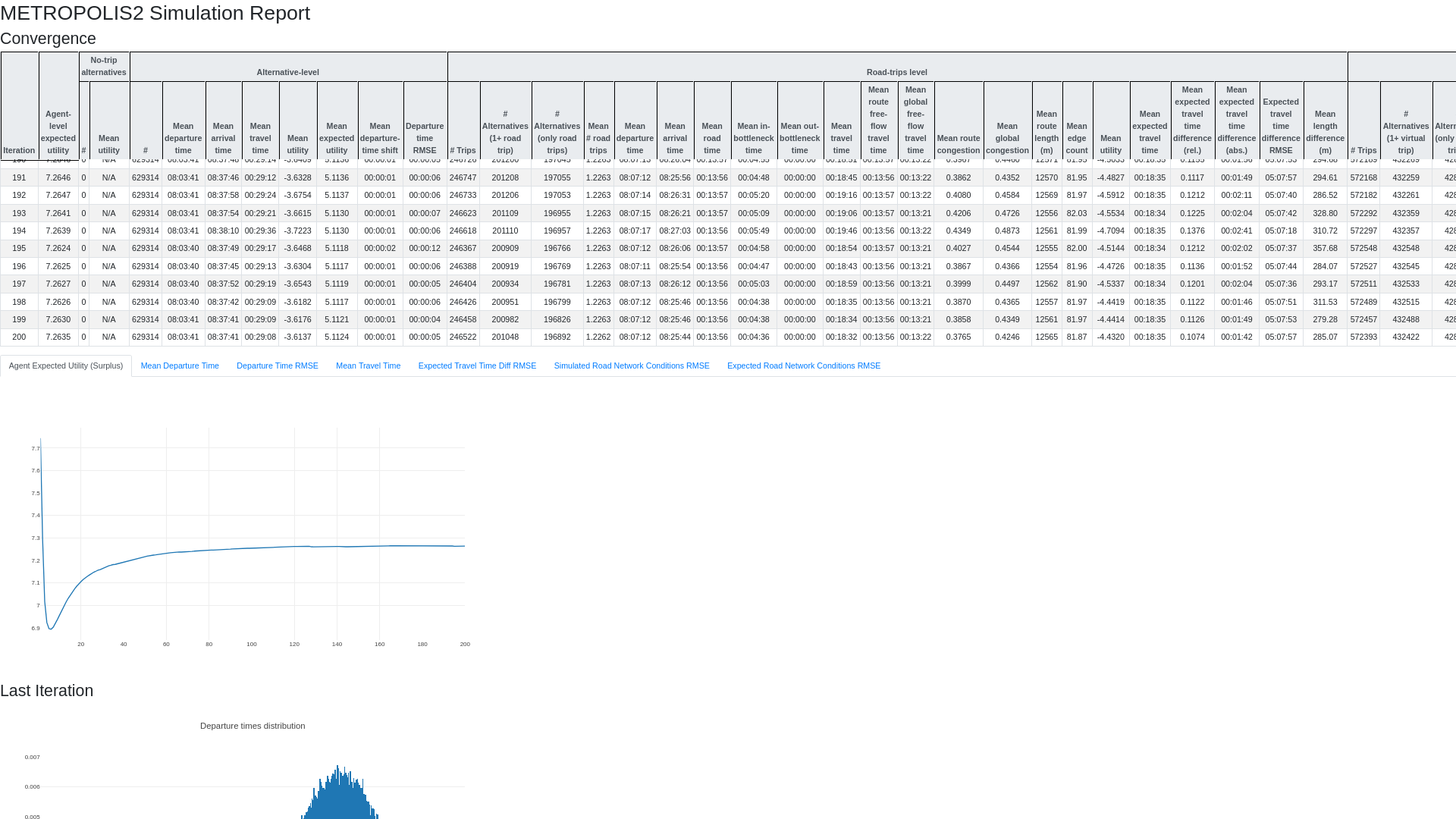
HTML Report
- Table of aggregate results by iterations
- Graphs of convergence through iterations
- Graphs of departure-time / arrival-time distribution for last iteration
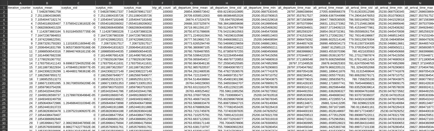
Iteration Results
- Parquet or CSV file
- 1 row for each iteration; 145 columns
- Aggregate results at the agent-level, road-trip level, virtual-trip level and road-network level
- Same variables as in the HTML report (with standard-deviation, minimum and maximum)
Route vs Global Free-Flow Travel Time
- Route free-flow travel time: no-congestion travel time on the route that was taken
- Global free-flow travel time: no-congestion travel time on the fastest possible route
- Route / Global congestion: share of travel-time spent in congestion, relative to route / global free-flow travel time
Population Results
All the results are specific to the last iteration
agent_results.{parquet,csv}: results at the agent-leveltrip_results.{parquet,csv}: results at the trip-levelroute_results.{parquet,csv}: detailed itineraries for the road trips
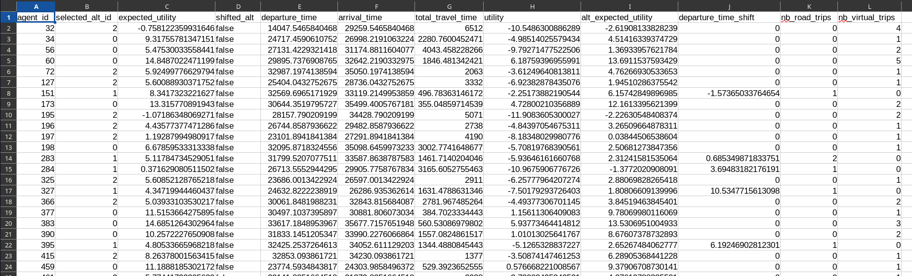
Agent Results
- Parquet or CSV file
- 1 row for each agent; 12 columns
- Results specific to the agents and their selected alternative
Utility Indicators (1/4)
-
utility: Simulated utility, based on the selected alternative $j$ and departure time $\tau$: $V^{\text{sim}}_{j}(\tau)$ -
alt_expected_utility: Expected utility of the departure-time choice of the selected alternative $j$: $\mathbb{E}_{\varepsilon}[\max_{\tau} U_j(\tau)]$ -
expected_utility: Expected utility of the alternative choice: $\mathbb{E}_{\varepsilon}[\max_{j} U_j]$
Utility Indicators (2/4)
Example with a deterministic alternative-choice model and a constant departure time
-
utility: Simulated utility, based on the selected alternative $j$, departure time $\tau$ and simulated travel times: $V^{\text{sim}}_{j}(\tau)$ -
alt_expected_utility: Expected utility, based on the selected alternative $j$, departure time $\tau$ and expected travel times: $V^{\text{exp}}_{j}(\tau)$ -
expected_utility: Expected utility, based on the selected alternative $j$, departure time $\tau$ and expected travel times: $V^{\text{exp}}_{j}(\tau)$
When the simulation has converged: $V^{\text{sim}}_j(\tau) \approx V^{\text{exp}}_j(\tau)$
Utility Indicators (3/4)
Example with a Logit alternative-choice model and a Continuous Logit departure-time choice model
-
utility: Simulated utility, based on the selected alternative $j$, departure time $\tau$ and simulated travel times: $V^{\text{sim}}_{j}(\tau)$ -
alt_expected_utility: Logsum of departure-time choice for the selected alternative $j$ \[ \bar{U}_j \equiv \mathbb{E}_{\varepsilon}[\max_\tau U_j(\tau)] = \mu \ln \int_{t^0}^{t^1} e^{V_j^{\text{exp}}(\tau) / \mu} \text{d} \tau + \mu \cdot 0.577 \] -
expected_utility: Logsum of alternative choice ("logsum of logsum") \[ \mathbb{E}_{\varepsilon}[\max_j U_j] = \mu \ln \sum_j e^{\bar{U}_j / \mu} + \mu \cdot 0.577 \]
Utility Indicators (4/4)
Which one to use (e.g., for cost-benefit analysis)?
-
utility: not really adapted when using random-utility models (the random perturbations $\varepsilon$ are omitted); recommended when using deterministic models (including models with drawn epsilons) -
alt_expected_utility: intermediate indicator, useful in some special cases only expected_utility: recommended when using random-utility models (it depends on the range of alternatives available, not just the realized choice: two identical agents always have the sameexpected_utilitybut they can have differentutilityif their uniform draws differ)
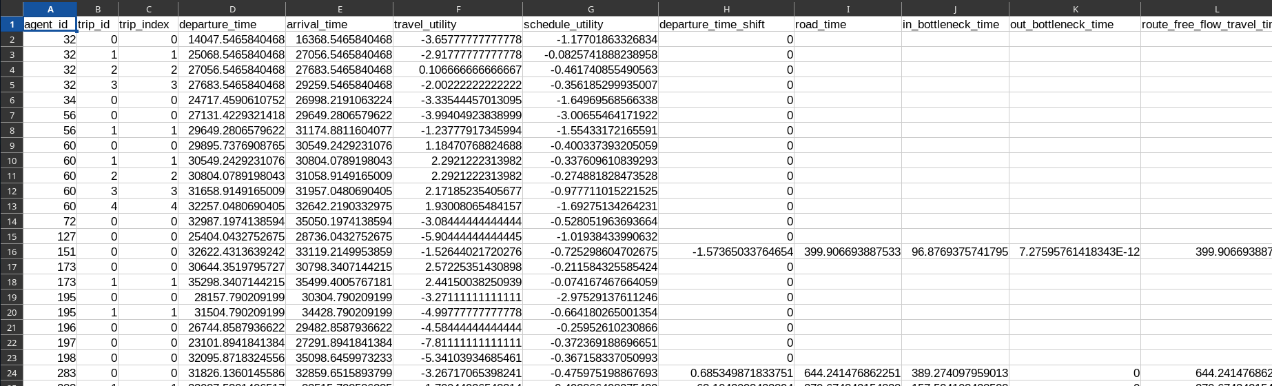
Trip Results
- Parquet or CSV file
- 1 row for each selected trip (road or virtual); 19 columns
- 11 columns are specific to road trips
Route Results
- Parquet or CSV file
- 1 row for each edge taken during road trips; 6 columns
- Detailed itinerary followed by the agents, as a list of edges with entry and exit time
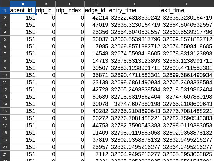
Route Results
Theroute_results.{csv,parquet} output file allows to show the detailed itinerary of an agent.
Route Results
Theroute_results.{csv,parquet} output file allows to show a video of the vehicle movements.
Road-Network Results
Three files for the road-network conditions (edge-level travel-time functions):
net_cond_sim_edge_ttfs.{parquet,csv}: last iteration, simulatednet_cond_exp_edge_ttfs.{parquet,csv}: last iteration, expectednet_cond_next_exp_edge_ttfs.{parquet,csv}: next iteration, expected
One extra file:
skim_results.json.zst: OD-level (expected) travel-time functions
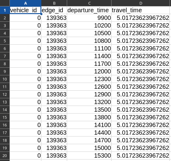
Network Conditions File Format
- Parquet or CSV file
- Number of rows: # edges × # breakpoints × # vehicle types
- Departure-time and travel-time breakpoints for each edge and vehicle type
- Departure-time breakpoints with simulated period [6 a.m., 10 a.m.] and recording interval 20 min.: [06:00, 06:20, 06:40, 07:00, 07:20, ..., 09:20, 09:40, 10:00]
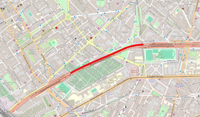
Network Conditions Map
When merged with the edges' geometries, the network conditions can be plotted on a map.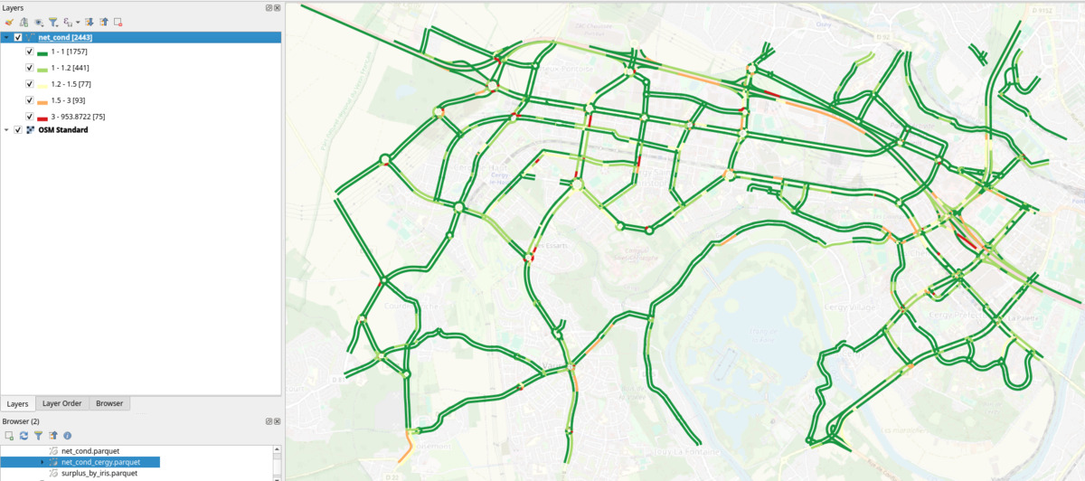
Starting Simulation from Network Conditions
- Default: use free-flow conditions as expected network conditions for the first iteration
- Initial network conditions can be given as input
- Input file format is the same as network conditions output file format
						{
								"input_files": {
										"agents": "agents.csv",
										"alternatives": "alts.csv",
										"trips": "trips.csv",
										"edges": "edges.csv",
										"vehicle_types": "vehicles.csv",
										"road_network_conditions": "net_cond_next_exp_edge_ttfs.csv"
								},
								"output_directory": "output",
								"period": [
										25200.0,
										28800.0
								],
								"road_network": {
										"recording_interval": 60.0,
										"spillback": false,
										"max_pending_duration": 0.0
								},
								"max_iterations": 100,
								"init_iteration_counter": 100,
								"saving_format": "CSV",
								"learning_model": {
										"type": "Exponential",
										"value": 0.4
								}
						}
parameters.json
Skim Results
- Travel-time function for each origin-destination pair in the population input (road trips)
- The travel-time functions are the one used in the demand model for the last iteration
- File format: compressed JSON for now; Parquet or CSV in a future update
Tasks
-
Go through Chapter 2 and Chapter 3 of Lucas Javaudin's PhD Thesis:
https://lucasjavaudin.com/research/phd-thesis/javaudin_lucas_phd_manuscript-final.pdf
- Go back to the slides of this session so that you have a global understanding of METROPOLIS2
- Build a small simulation from scratch