Impact of Low-Emission Zones on Spatial and Economic Inequalities using a Dynamic Transport Simulator
Lucas Javaudin
THEMA PhD Seminar – 2023-03-30
Introduction
Context
- Each year 430,000 Europeans die prematurely due to air pollution (European parliament)
- Air pollution is mainly caused by nitrogen oxides (NOx) emitted by road vehicles
- Popular instrument to improve air quality: Low Emission Zones (LEZ)
Low Emission Zones
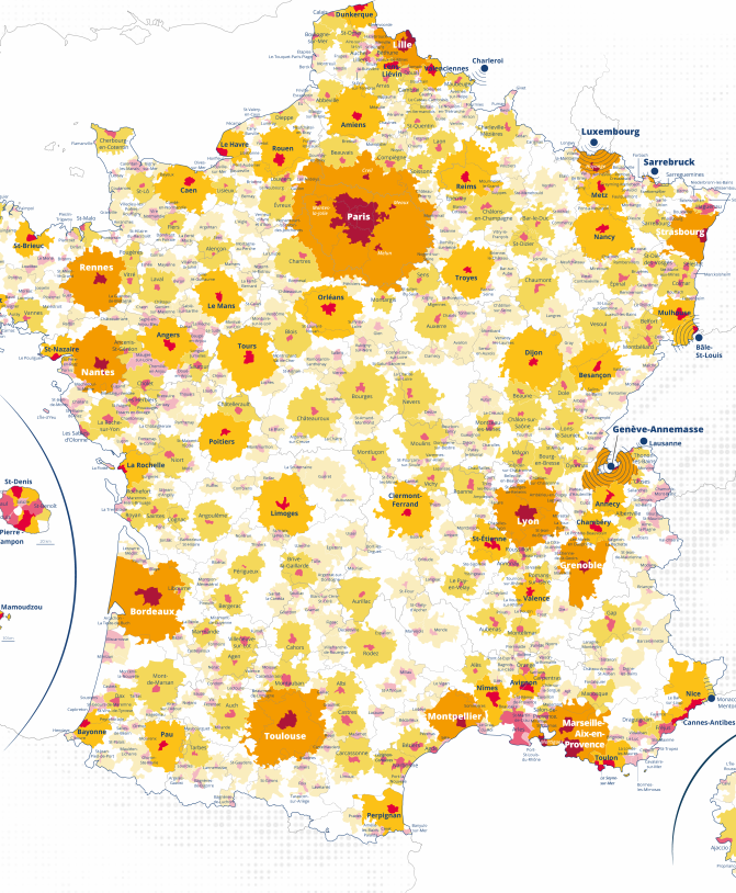
- In Europe, LEZs have been implemented in hundreds of cities
- Starting in 2025, LEZs will be mandatory for French cities with more than 150,000 inhabitants
- Benefits of LEZs: reducing local and global air pollution, congestion and noise pollution
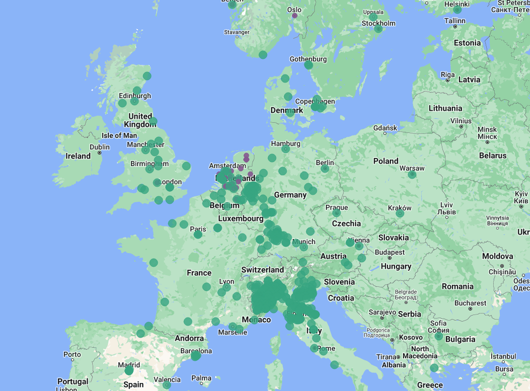
Source: urbanaccessregulations.eu
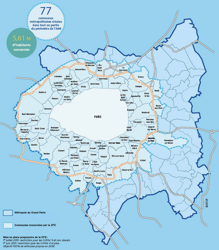
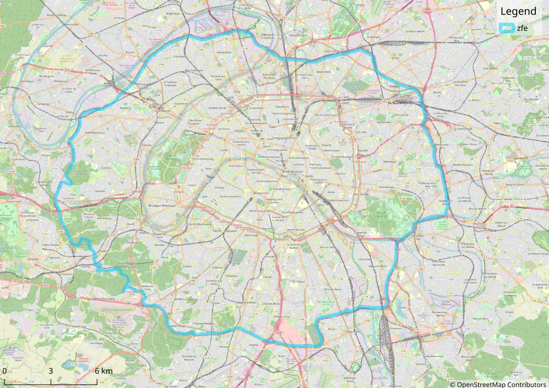
Paris' Low Emission Zone
- More than 5 millions inhabintants are leaving in the LEZ
- The LEZ represent around 10 % of the Île-de-France's road network
- June 2021: Crit'air 4 vehicles and worse are banned (11 % of the fleet)
- July 2023: Crit'air 3 vehicles and worse are banned (34 % of the fleet)
Heterogeneous Effects
Not all individuals are affected in the same way by a Low
Emission Zone.
Sources of heterogeneity:
Sources of heterogeneity:
- Household living inside the LEZ vs outside the LEZ
- High income vs low income
- Owner of a clean car vs a polluting car
- Car driver vs public-transit user
Metropolis: A Transport Simulator
We introduce a new transport simulator with the following
characteristics:
- based on economic theory (utility maximization)
- multi-modal (it includes private and public transports)
- dynamic (congestion is time-dependent and departure times are endogenous)
- mesoscopic (vehicle flow are aggregated at link-level)
- agent-based (each individual is modeled as an autonomous entity)
- adapted to large-scale scenario (up to 1 million roads and 10 millions agents)
Literature Review
Impact of Low Emission Zones:
Agent-based transport simulators:
- Empirical evaluation: focus on environmental impact, ambiguous effect (Holman et al., 2015; Wolff, 2014; Margaryan, 2021)
-
Ex-ante evaluation:
- Carslaw and Beevers (2022): approached based on traffic flow data, using an emission and dilution model
- Dias et al. (2016): macroscopic transport model
- Bok el al. (2022): agent-based model, focus on freight transport
Agent-based transport simulators:
- MATSim (Axhausen et al., 2016): activity-based, behavior-oriented
- SimMobility (Adnan et al., 2016): activity-based, hierarchical discrete choice modeling
Contributions
- Development of a new agent-based transport simulator: Metropolis
- Calibration to Paris' urban area (work in progress)
- Evaluation of the Low Emission Zone of the Métropole du Grand Paris (work in progress)
Outline
- Presentation of the transport simulator Metropolis
- Application to Paris' urban area
- Preliminary results: aggregate results, winners and losers from the LEZ
Metropolis
Objectives
- Find a Nash equilibrium for a representative day in an urban area
- Equilibrium: no agent can increase his / her utility by changing mode, departure time or route, given the expected traffic congestion
- Compare baseline equilibrium with the equilibrium in other scenarios (e.g., new transit lines, Low Emission Zone, speed-limit change)
-
Results:
- Aggregate impact of the policy on travel times, utilities, congestion, etc.
- Spatial impact (e.g., city center vs suburbs)
- Social impact (e.g., poor vs rich households)
Input of the Model
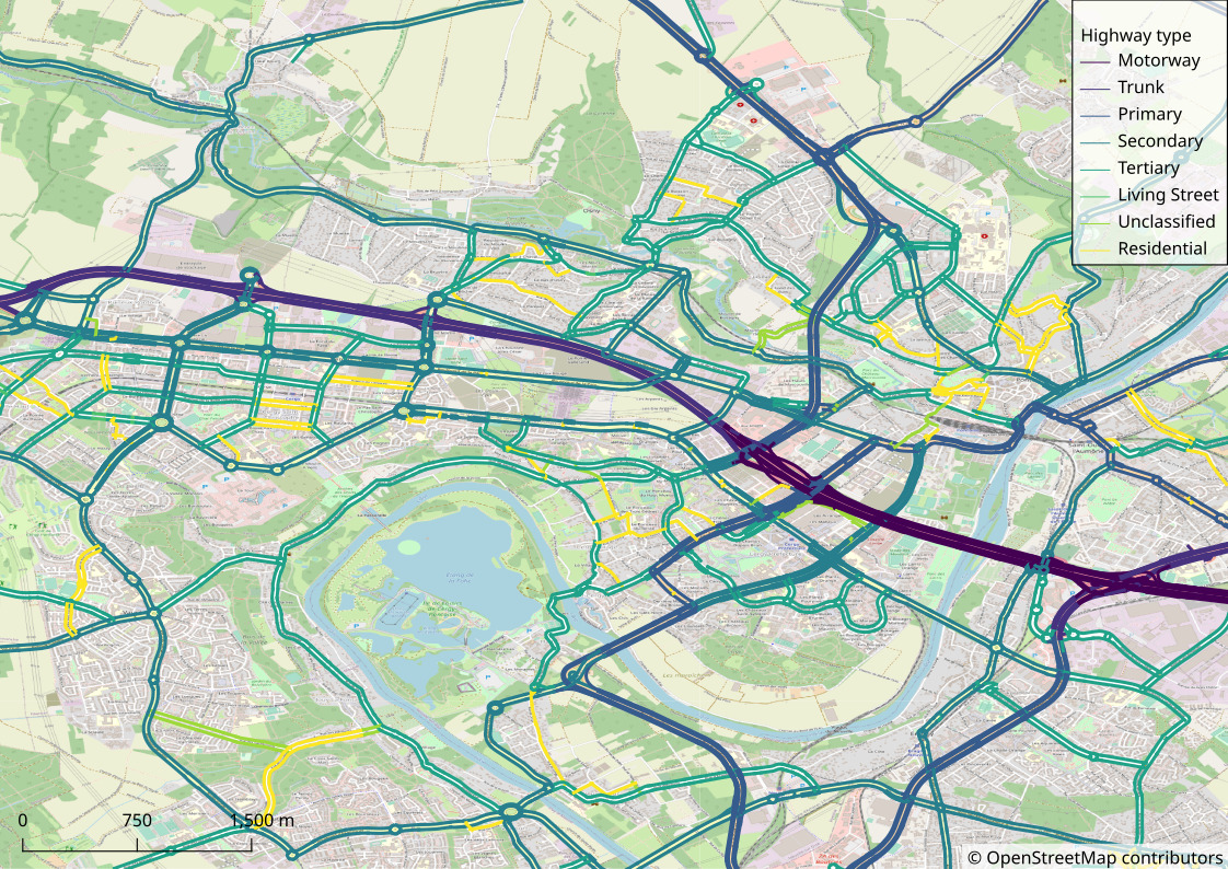
Road network
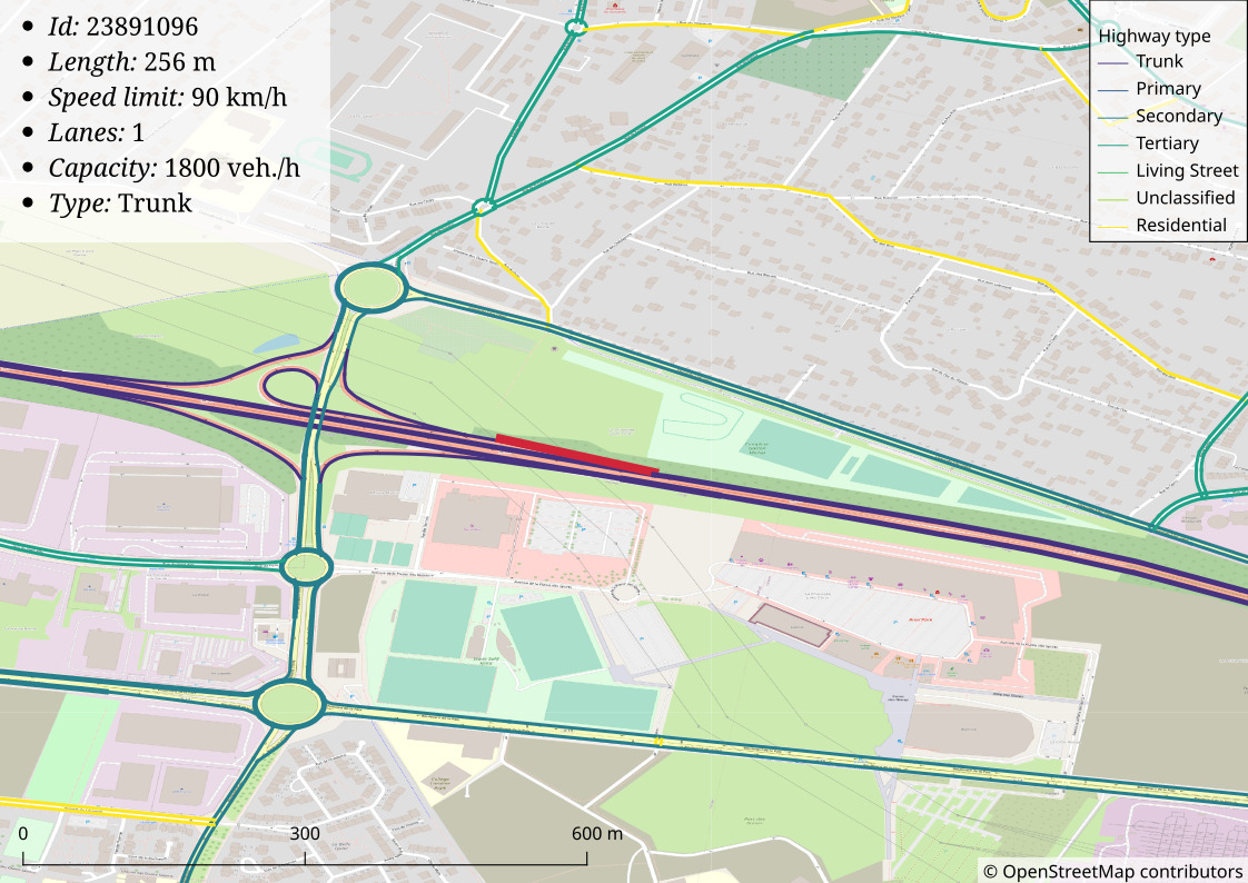
Vehicle types:
- Headway between two vehicles
- Passenger car equivalent
- Speed function (representing speed limits)
- Road restrictions
Input of the Model
Population
List of agents with the characteristics of their trips (for each
mode available):
- Origin and destination
- Vehicle type
- Travel-utility model (a function of the travel time; e.g., proportional to the value of time)
- Schedule-utility model (a function of the departure and arrival time; e.g., alpha-beta-gamma model)
Basic Principle
- Metropolis is an iterative model
- At each iteration, four models are run successively (network skims computation, pre-day model, within-day model and day-to-day model)
- The simulation stops when a convergence criteria is met or when the maximum number of iterations is reached
Network skims computation
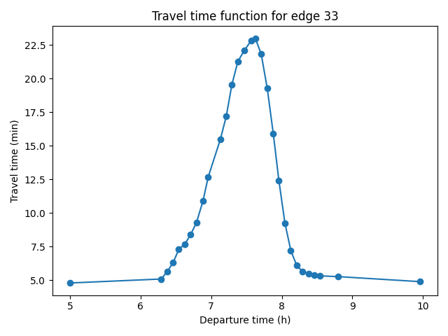
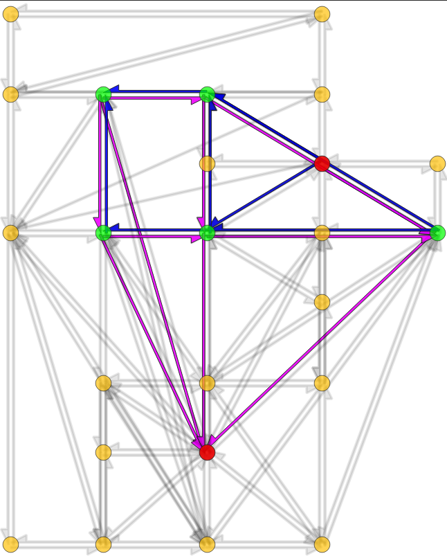
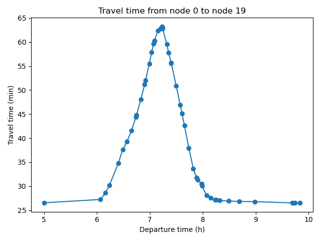
- Input: time-dependent travel-time function for each road of the road-network graph
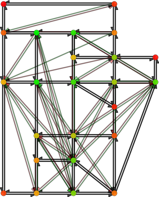
- Step 1: compute a time-dependent Hierarchy Overlay of the graph
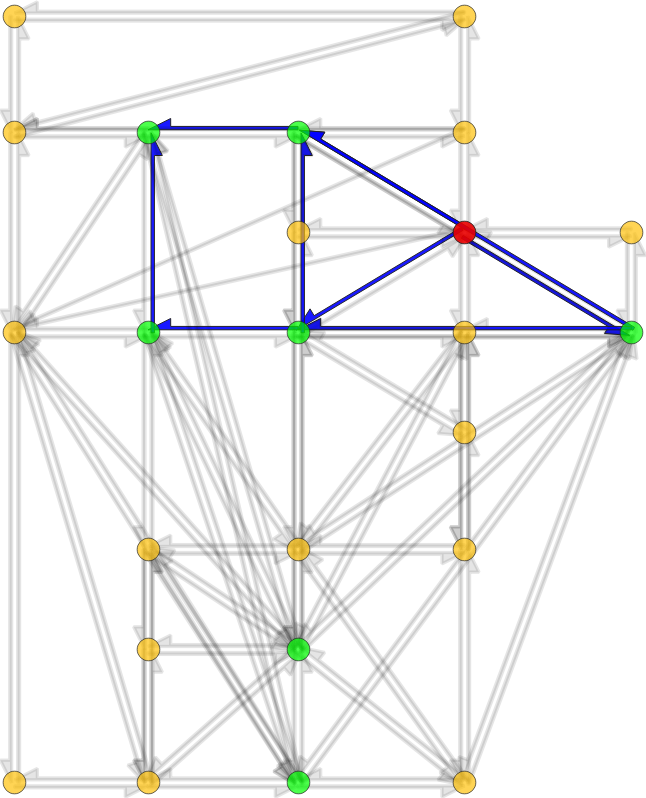
- Step 2: compute search spaces for each origin and destination node
- Step 3: compute profile queries for each origin-destination pair
- Output: time-dependent travel-time function for each origin-destination pair (with at least one trip)
Geisberger, R. and Sanders, P., 2010. Engineering time-dependent
many-to-many shortest paths computation. In
10th Workshop on Algorithmic Approaches for Transportation
Modelling, Optimization, and Systems (ATMOS'10). Schloss Dagstuhl-Leibniz-Zentrum fuer Informatik.
Pre-Day Model
- Input: time-dependent travel-time function for each origin-destination pair
- Output: mode, departure-time and route chosen by each agent
- Backward induction process, based on trip utility
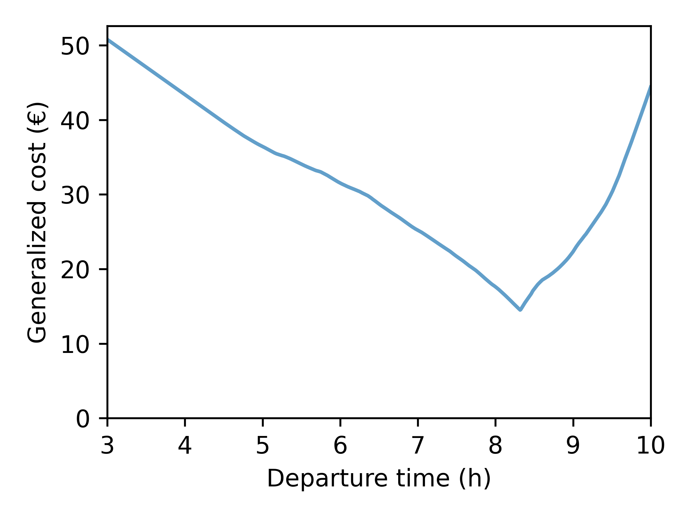
Bottleneck Equation
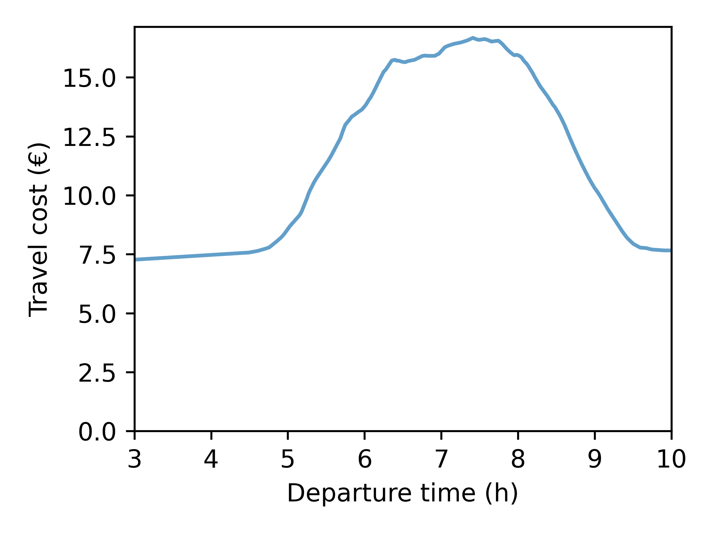
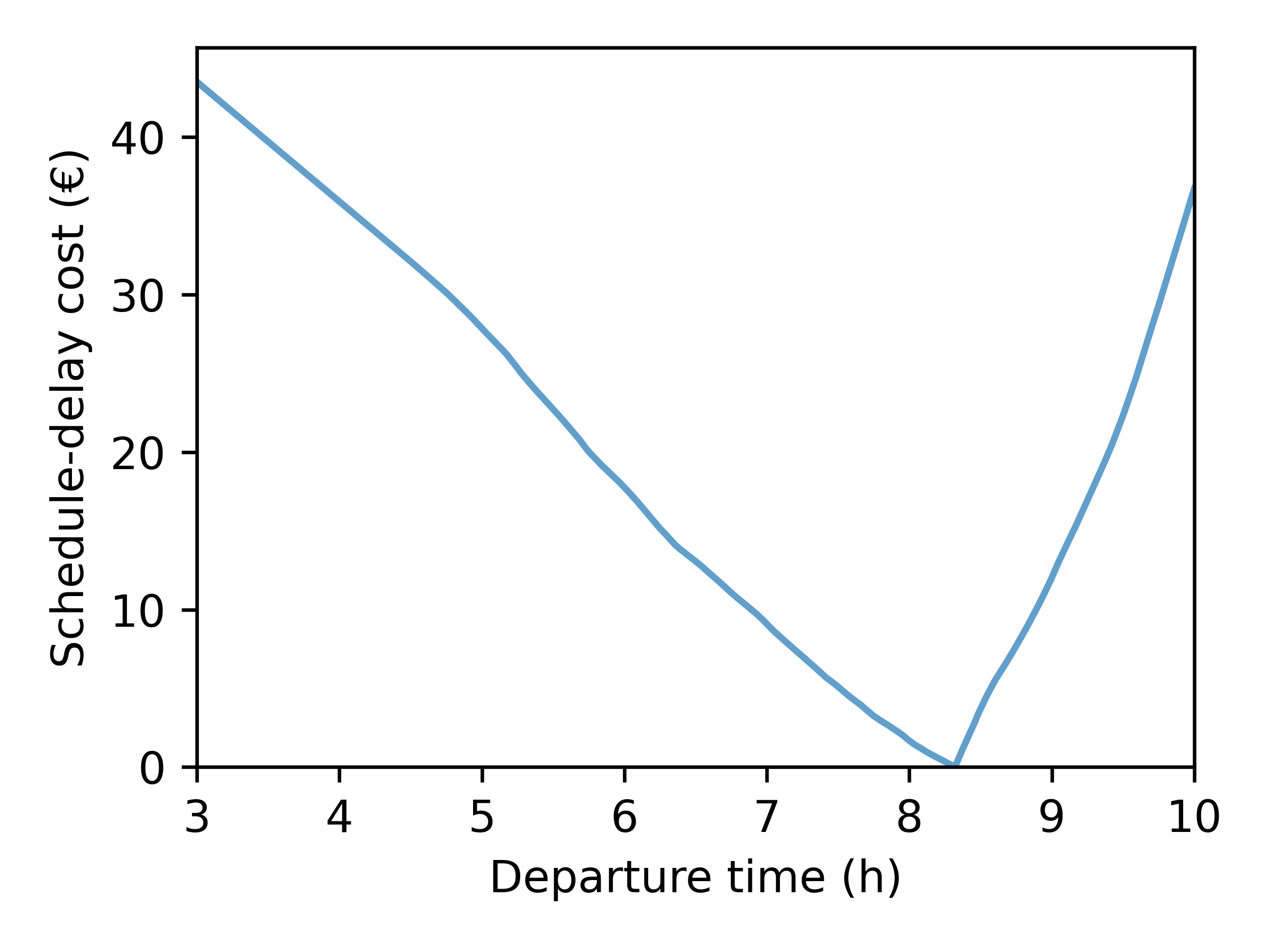
A trip generalized cost (minus utility) is \[ c(t_d, t_a) =
\underbrace{\alpha \cdot (t_a - t_d)}_{\text{travel cost}} +
\underbrace{\beta \cdot [t^* - t_a]_+ + \gamma \cdot [t_a -
t^*]_+}_{\text{schedule-delay cost}} \]
- \( t_d, t_a \): departure time, arrival time
- \( \alpha \): value of time
- \( t^* \): desired arrival time
- \( \beta, \gamma \): penalty for early, late arrival
+
=
Pre-Day Model
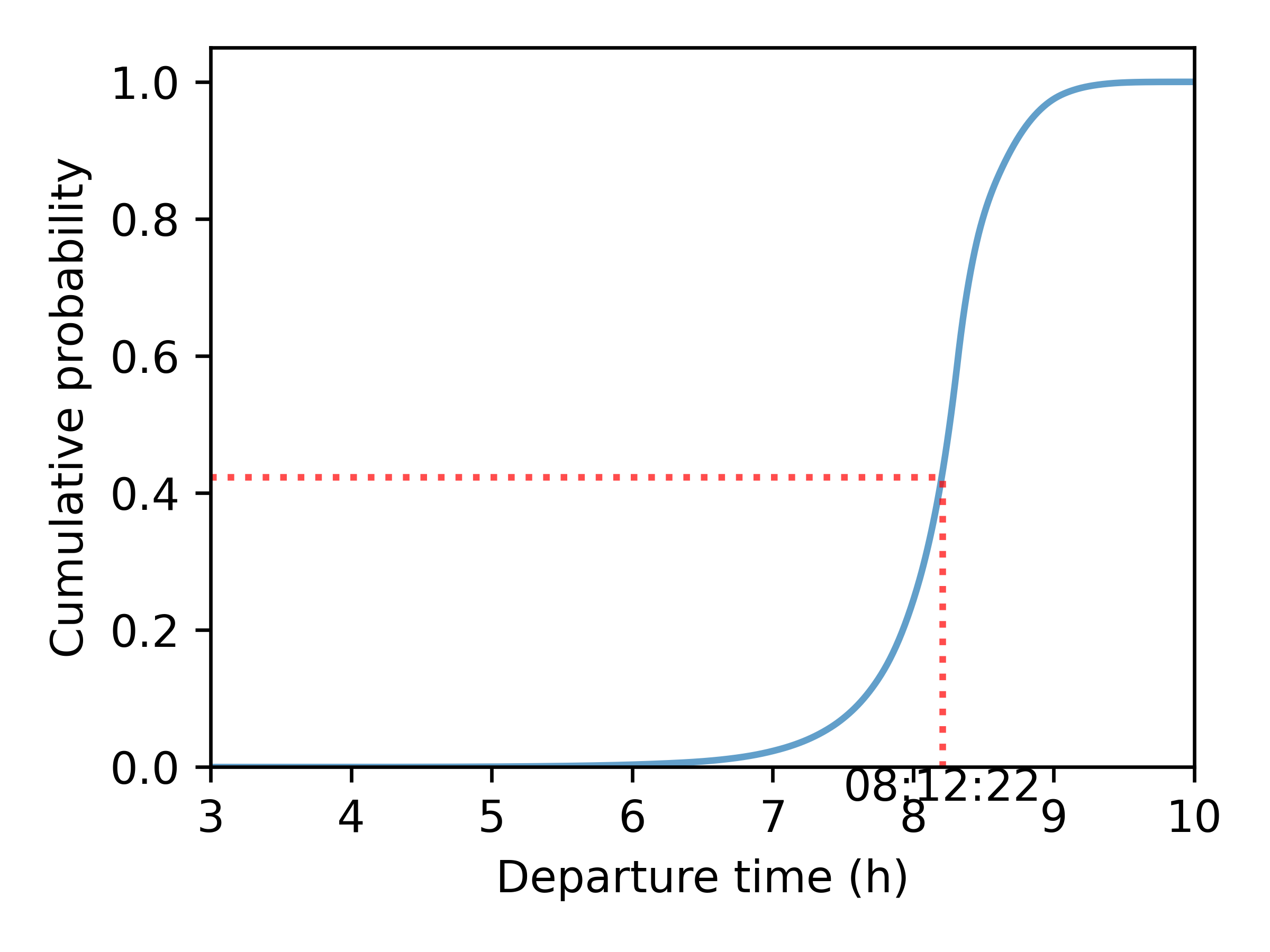
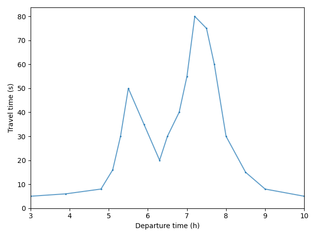
Departure-Time Choice
A Continuous Logit Model combined with inverse transform sampling is used to simulate a departure time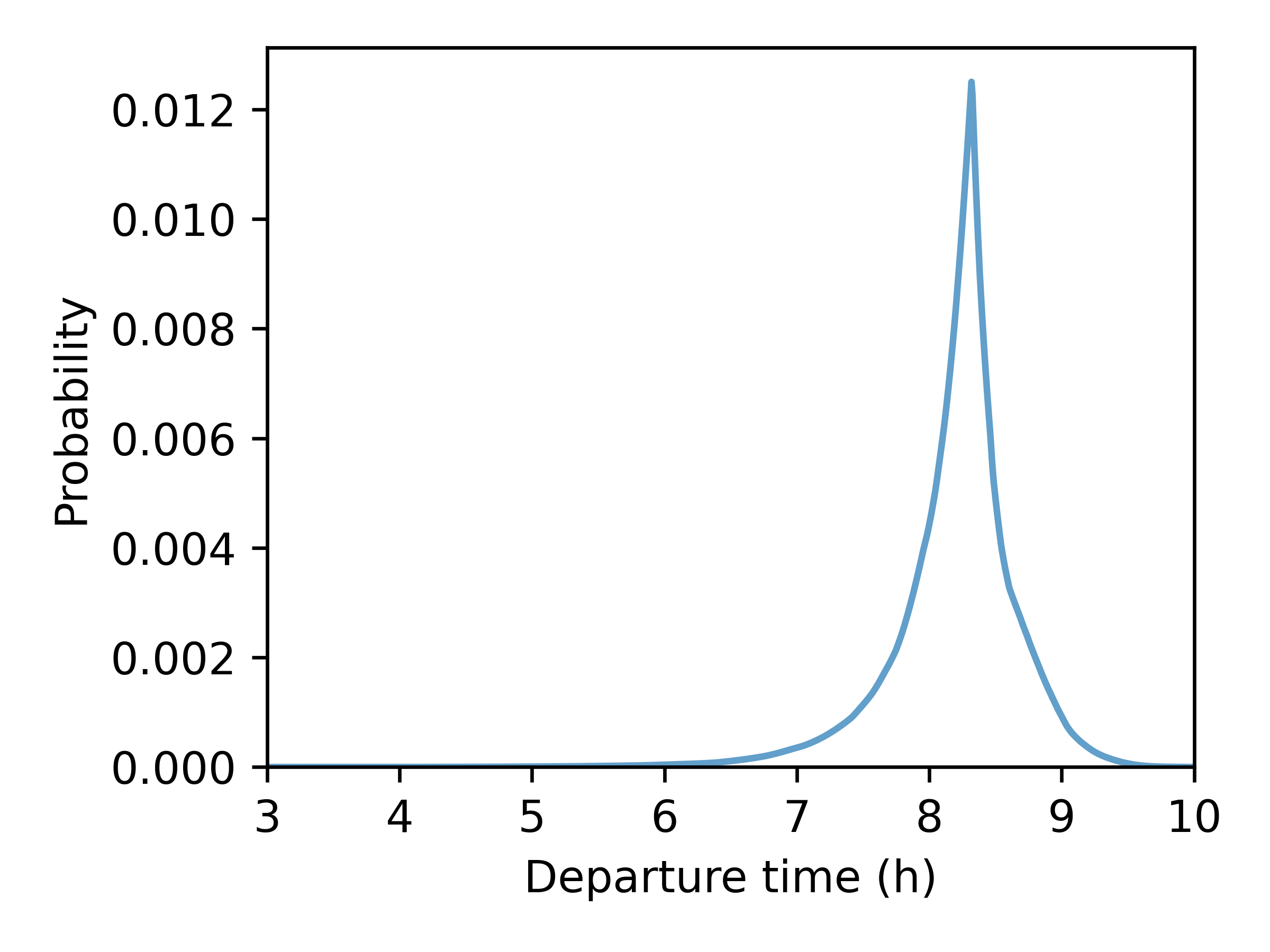
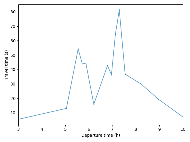
Within-Day Model
- Input: Chosen mode, departure time and route of each agent
- Event-based model: Agents' actions are simulated in a chronological order
- Output: Edges' travel-time functions
| Time | Event |
|---|---|
| 03:00:03 | Agent 91735 leaves origin through edge 317770 |
| 03:00:11 | Agent 111697 leaves origin through edge 161026 |
| 03:00:27 | Agent 111697 takes edge 161020 |
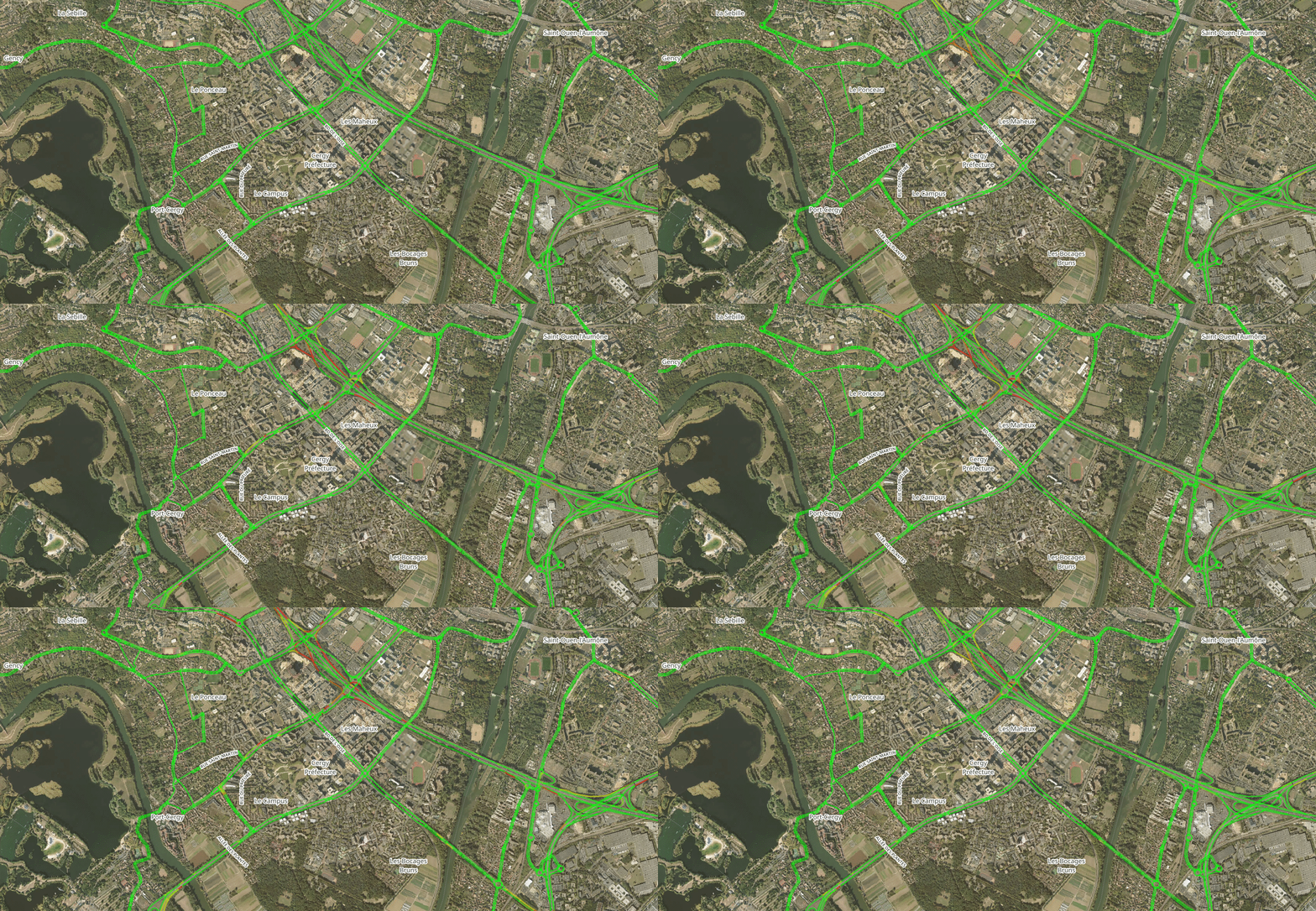
Congestion Modeling
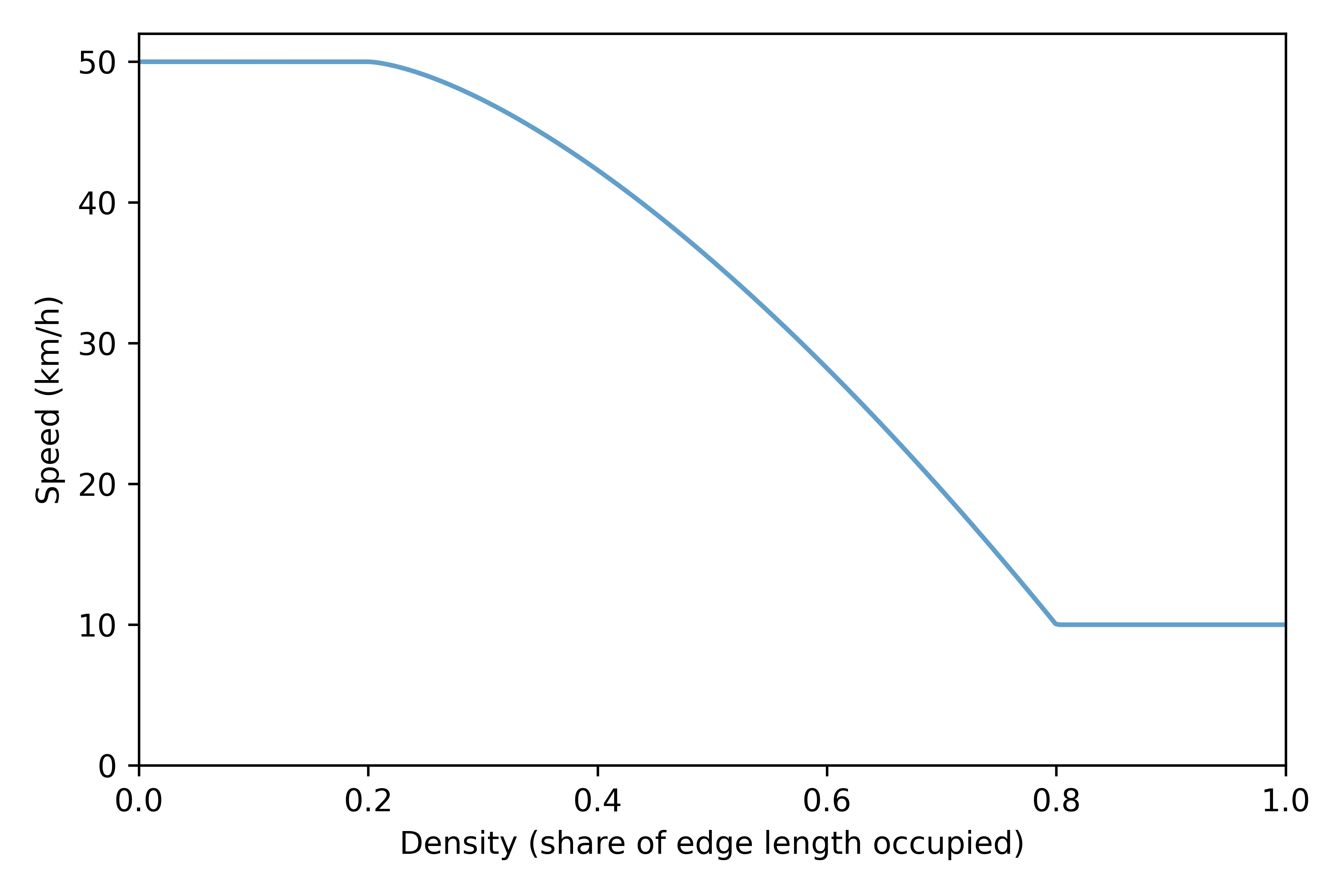
- Speed-density function
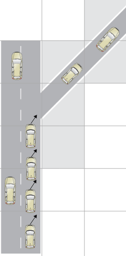
- Traffic bottleneck
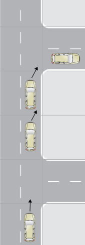
- Queue propagation
Day-to-Day Model
- Input: Expected and simulated edges' travel-time functions
- Learning process based on Markov decision processes
- Output: Expected edges' travel-time functions for next iteration

\[ {tt}^e_{\tau + 1} = \lambda \cdot {tt}^e_{\tau} + (1 -
\lambda) \cdot {tt}^s_{\tau} \]
Convergence
Ways to check convergence to a Nash equilibrium:

- Choices do not change
- Expected congestion does not change
- Expected congestion matches simulated congestion
- No proof on stability and uniqueness of equilibrium
Example Applications
- Air pollution (Le Frioux, de Palma, Blond)
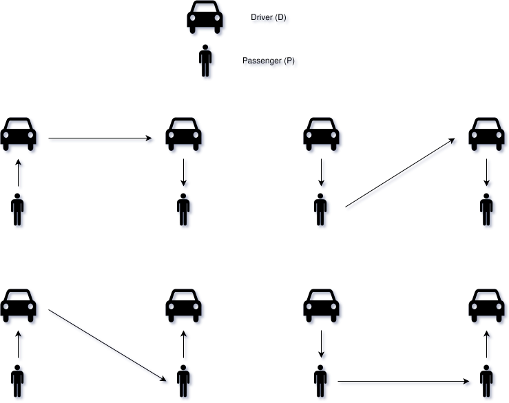
- Ride-sharing (de Palma, Delle Site, Ghoslya, Javaudin)
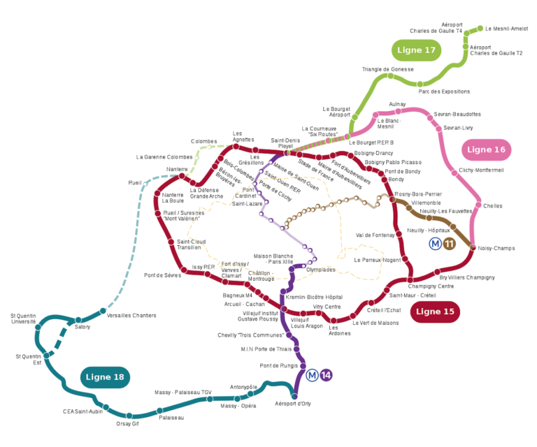
- Public transit and Grand-Paris Express evaluation (Javaudin)
- Automatic calibration for any French cities with various open datasets


Application
Introduction
- Scope: Île-de-France, trips by car between 3AM and 10AM, all purposes, representative working day
-
Three scenarios:
- No-LEZ simulation: Simulation without the Low Emission Zone
- LEZ-2021 simulation: Crit'air 4 and 5 are forbidden
- LEZ-2023 simulation: Crit'air 3, 4 and 5 are forbidden
-
Limits:
- No mode choice
- No car-ownership model
- Time restrictions are not taken into account
- Cheating and exceptions are not considered
Input: Road network
- Source: OpenStreetMap
- Highway types: motorway, trunk, primary, secondary, tertiary, living street, unclassified and residential
- Living streets, unclassified and residential roads are discarded when not used
- Final network has 40 852 km of roads (out of 91 859 km in the full network)
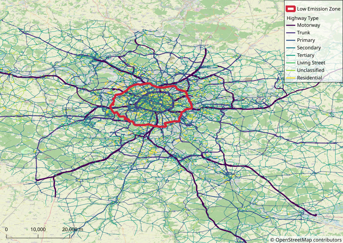
Input: Road network


Input: Population
- Generation of a synthetic population using Hörl and Balac (2021)
- Data sources: INSEE census, household travel survey, FiLoSoFi (household income), BD-TOPO (buildings data), SIRENE (entreprise census) and BPE (service and facility census)
- Simulated household-level characteristics: car availability, bike availability, income
-
Simulated individual-level characteristics:
- all activities performed during a day (home, work, education, leisure, shopping, other) with the activity duration and exact location
- age, employment status, sex, socio-professional category, driving license, public-transit subscription
- Final population: 193 235 agents, with 254 585 trips
Hörl, S. and Balac, M., 2021. Synthetic population and travel demand for Paris and Île-de-France based on open and publicly available data. Transportation Research Part C: Emerging Technologies, 130, p.103291.
Input: Population
Example agent
Household
- Members: 2
- Car available: 1
- Bike available: 2
- Disposable income: 13 101 euros (monthly)
Individual
- Age: 60
- Employed: Yes
- Sex: Woman
- Socio-professional class: 3 (Cadres et professions intellectuelles supérieures)
- Driving license: Yes
- Public-transit subscription: No
Input: Population
Example agent
Activities
- Home until 07:33
- Work from 09:03 to 12:43
- Leisure from 12:48 to 13:28
- Work from 13:33 to 20:03
- Home from 20:38 to 21:03
- Leisure from 23:23 to 23:33
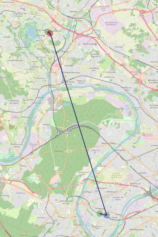
Input: Population
Vehicle Types
- Data: Statistics on the vehicle fleet from the French Ministry of Transport (2021)
- INSEE Communes level
- A vehicle is randomly drawn for each agent based on the vehicle fleet from his / her home city
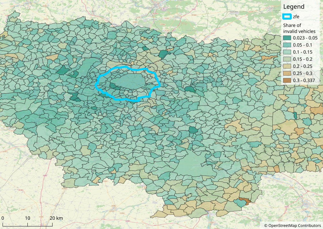

A Note on Calibration
- Values to estimate or calibrate: road capacities, agents' preferences (value of time, schedule-delay penalties), activities' desired arrival times
-
Three options:
- Use a value from the literature
- Estimate a value from revealed or declared preferences (e.g., from a travel survey data)
- Calibrate the value to match observed data (e.g., traffic counts, distribution of arrival times)
- In this work: road capacities and preferences are taken from the literature; desired arrival times are set to observed arrival times
Calibration
Travel time penalties at intersections are calibrated to match travel time distribution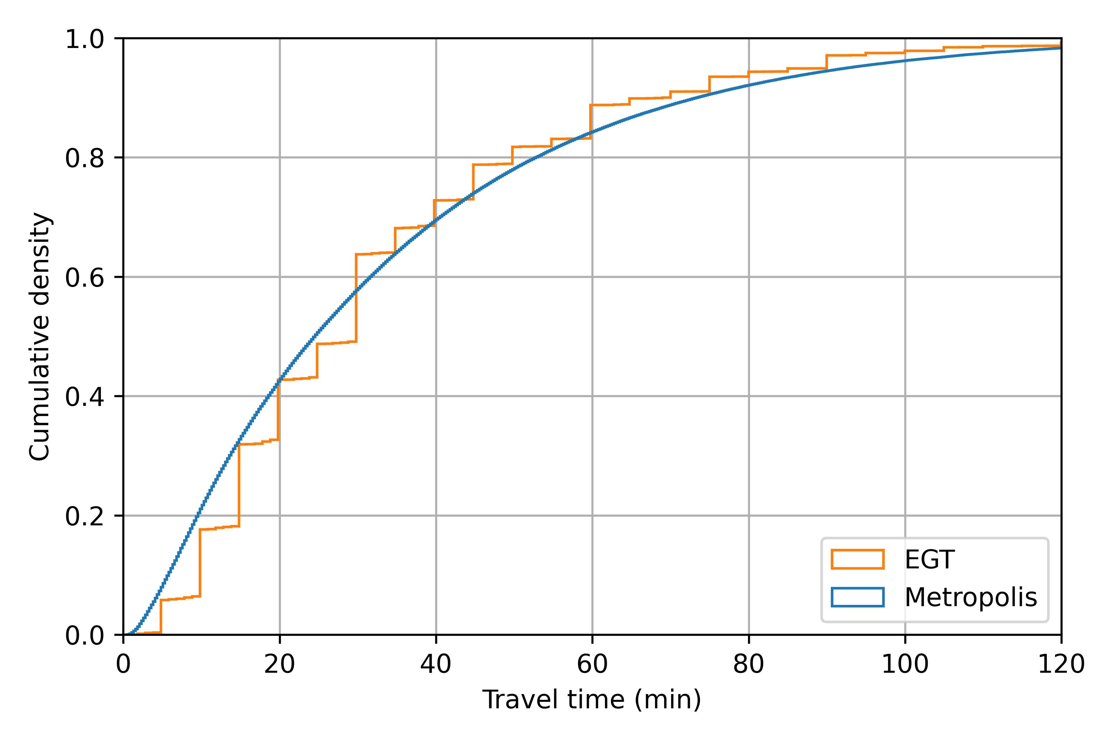
Calibration
Distribution of desired arrival times is calibrated to match arrival time distribution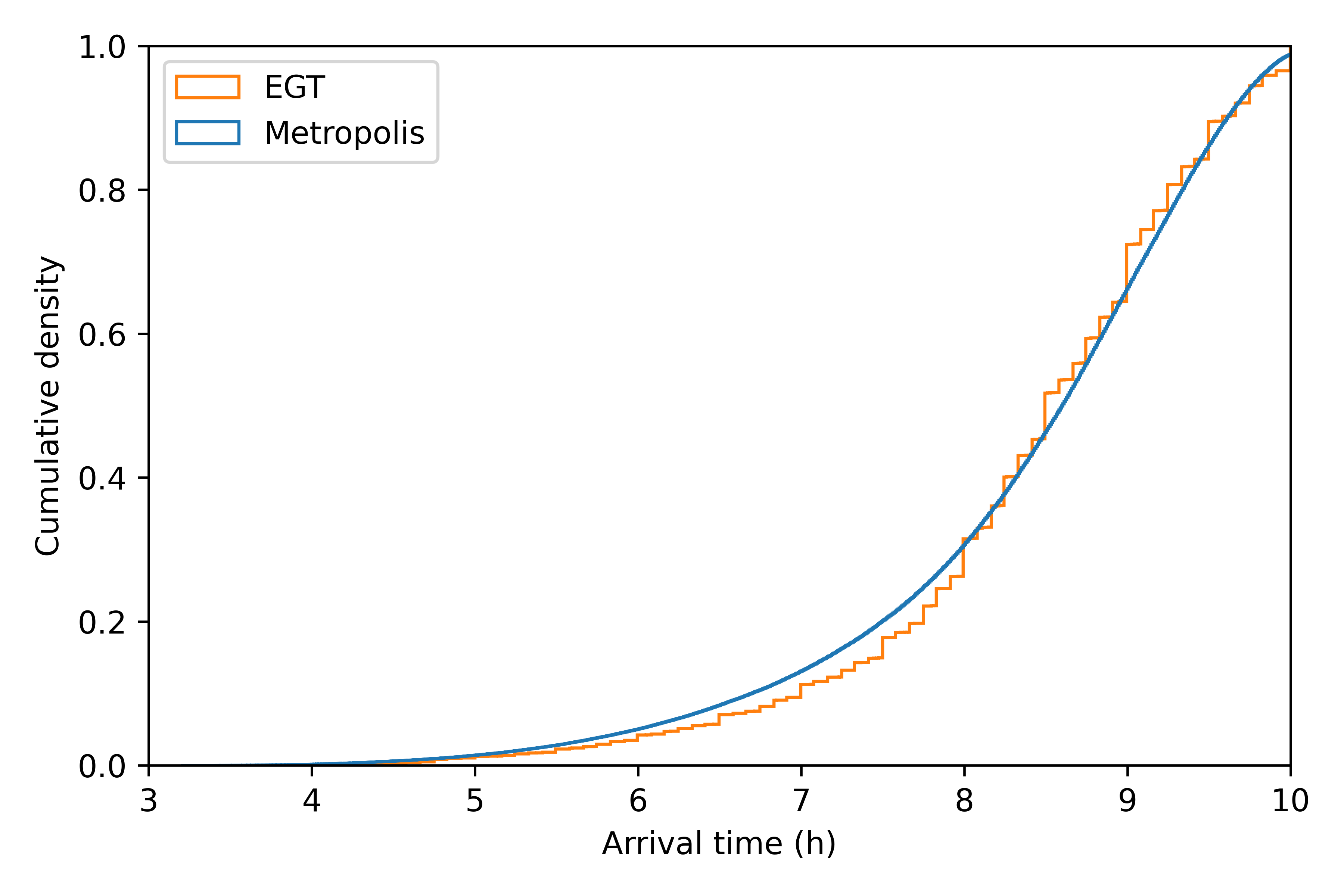
Results
Convergence
Choice stability
- Average departure-time shift (in absolute value) is 1.47 seconds (maximum is 105 seconds), at last iteration
- On average, the route used by each agent is the same as the one from the previous iteration for 98.12 % of its length, at last iteration


Convergence
Expected congestion stability
The average travel time anticipated is equal to 17 minutes and 19 seconds (\(\pm\)1s) for the last 35 iterations.
Convergence
Correctness of Anticipations
- EXPECT: relative difference between the anticipated and simulated travel times
- On average, agents under-estimate or over-estimate their travel time by 11.44 % (= 2'33''), at the last iteration

Aggregate Results
| No LEZ | LEZ-2021 | LEZ-2023 | |
|---|---|---|---|
| Departure time | 07:46:13 | 07:46:12 | 07:46:14 |
| Travel time | 19'00 | 18'37'' | 18'26'' |
| Route length (m) | 13 686 | 13 684 | 13 694 |
| Generalized cost (euros) | 10.26 | 10.02 | 9.93 |
Results by Segment
Three segments (in the LEZ-2023 scenario):
- Segment A: Trip starts or ends in the LEZ (48.2 %)
- Segment B: Trip does not start nor end in the LEZ / Clean vehicle (33.1 %)
- Segment C: Trip does not start nor end in the LEZ / Polluting vehicle (18.7 %)
Results by Segment
Travel time
| No LEZ | LEZ-2023 | Difference | |
|---|---|---|---|
| Segment A | 27'31'' | 26'22'' | –1'11'' |
| Segment B | 11'4'' | 11'0'' | –4'' |
| Segment C | 11'6'' | 11'7'' | +1'' |
Route length (m)
| No LEZ | LEZ-2023 | Difference | |
|---|---|---|---|
| Segment A | 16 182 | 16 178 | -4 |
| Segment B | 11 320 | 11 319 | -1 |
| Segment C | 11 446 | 11 504 | +58 |
| No LEZ | LEZ-2023 | Difference | |
|---|---|---|---|
| Segment A | 10.79 | 10.27 | -0.52 |
| Segment B | 5.33 | 5.30 | -0.03 |
| Segment C | 5.35 | 5.34 | -0.01 |
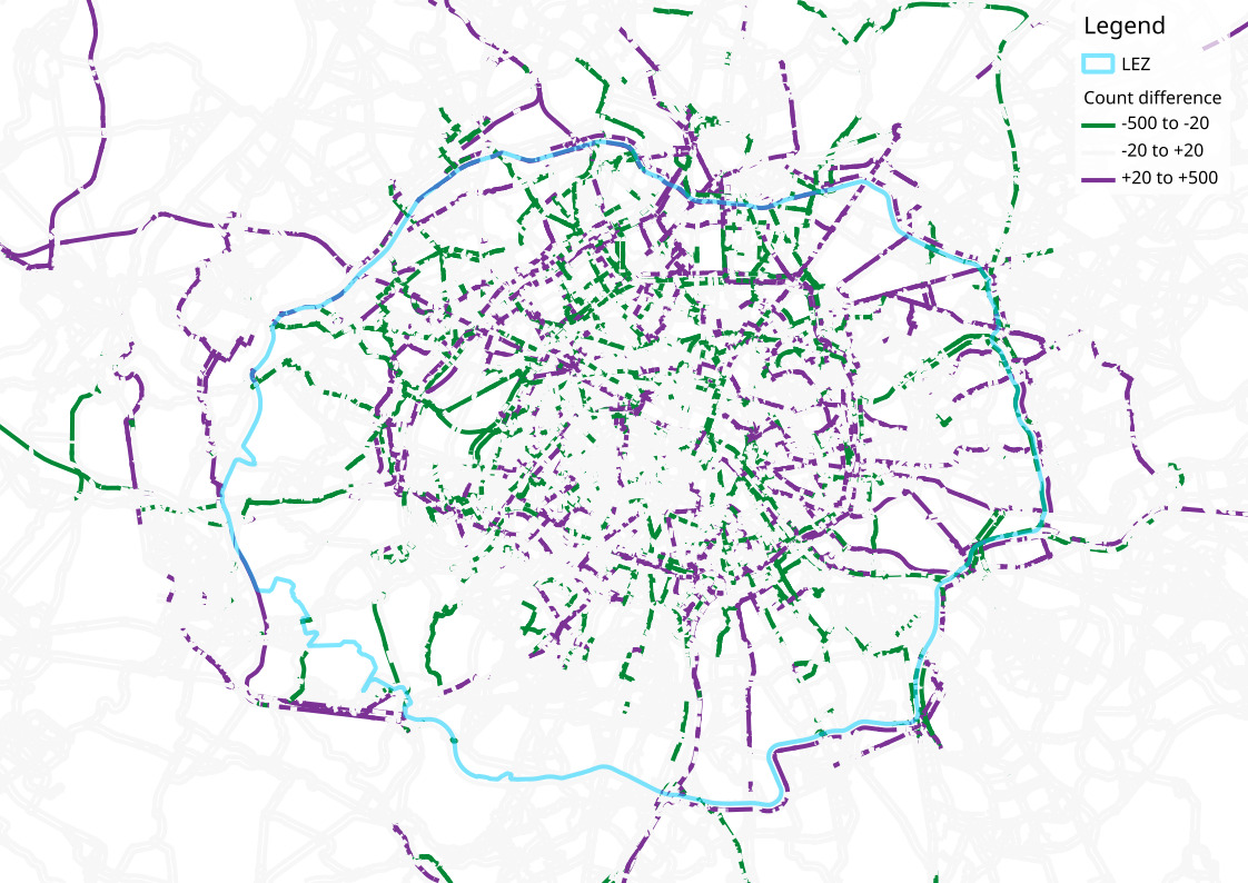
Traffic Counts Change


Traffic Counts Change
Conclusion
Conclusion
Results
Future works
- Metropolis is adapted to study the heterogeneous effect of a policy (such as a LEZ)
-
Paris' LEZ has
- a positive effect on the people living or working inside the LEZ
- an ambiguous effect of the people living and working outside of the LEZ, owning a clean car
- a negative effect of the people living and working outside of the LEZ, owning a polluting car
Future works
- Mode choice
- Car ownership
- Calibration and validation
- Improve convergence
- Additional results (results by demographic groups, air pollution)