Metropolis

André de Palma, Lucas Javaudin (CY Cergy Paris Université)

Société du Grand Paris – 2022-12-15

## Team

Scientific advisers:

<table>
								<tr>
									<th>Name</th>
									<th>Status</th>
									<th>Affiliation</th>
								</tr>
								<tr>
									<th>Araldo, Andrea</th>
									<td>Associate Professor</td>
									<td>Télécom SudParis, Institut Polytechnique de Paris</td>
								</tr>
								<tr>
									<th>Coulombel, Nicolas</th>
									<td>Associate Professor</td>
									<td>LVMT, École des ponts ParisTech</td>
								</tr>
								<tr>
									<th>Geroliminis, Nikolas</th>
									<td>Professor</td>
									<td>LUTS, École Polytechnique Fédérale de Lausanne</td>
								</tr>
								<tr>
									<th>Kilani, Moez</th>
									<td>Professor</td>
									<td>Université du Littoral Côte d'Opale</td>
								</tr>
								<tr>
									<th>Lindsey, Robin</th>
									<td>Professor</td>
									<td>Sauder School of Business, University of British Columbia</td>
								</tr>
								<tr>
									<th>Picard, Nathalie</th>
									<td>Professor</td>
									<td>BETA, University of Strasbourg</td>
								</tr>
								<tr>
									<th>Seshadri, Ravi</th>
									<td>Assistant Professor</td>
									<td>Technical University of Denmark</td>
								</tr>
							</table>

## History of the Project

<ul>
								<li class="fragment" data-fragment-index="0"><b>1997-2009:</b> Simulator v1 [C++] (de Palma, Marchal, Nesterov)</li>
								<li class="fragment" data-fragment-index="1"><b>2001-2009:</b> Interface for the simulator v1 [Java] (Marchal)</li>
								<li class="fragment" data-fragment-index="2"><b>2018-2021:</b> Web interface for the simulator v1 [Python Django] (Javaudin et al.)</li>
								<li class="fragment" data-fragment-index="3"><b>2021-:</b> Simulator v2 [Rust] (de Palma, Javaudin)</li>
								<li class="fragment" data-fragment-index="4"><b>2021-:</b> Interface for the simulator v2 [Python + JavaScript] (Javaudin et al.)</li>
							</ul>

Basic Principle

Metropolis is an iterative model
At each iteration, four models are run successively (network skims computation, pre-day model, within-day model and day-to-day model)
The simulation stops when a convergence criteria is met or when the maximum number of iterations is reached

Input of the Model

The input of Metropolis can be divided in three main categories:

Road network
Population (list of agents and their characteristics)
Simulation parameters

Id: 11484148
Purpose: Home to work
Origin: 951270127 (Cergy – Justice-Heuruelles)
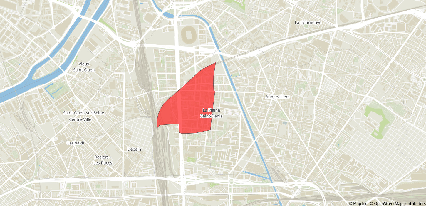
Destination: 930661102 (Saint-Denis – Plaine 02)
Age: 39
Sex: male
Employed: Yes
Socioprofessional class: 3 (executive)
Driving license: Yes
Monthly household income: 3369 €

Output of the Model

The output of Metropolis can be divided in four main categories:

Aggregate results (e.g., mean travel time, surplus)
Agent-specific results
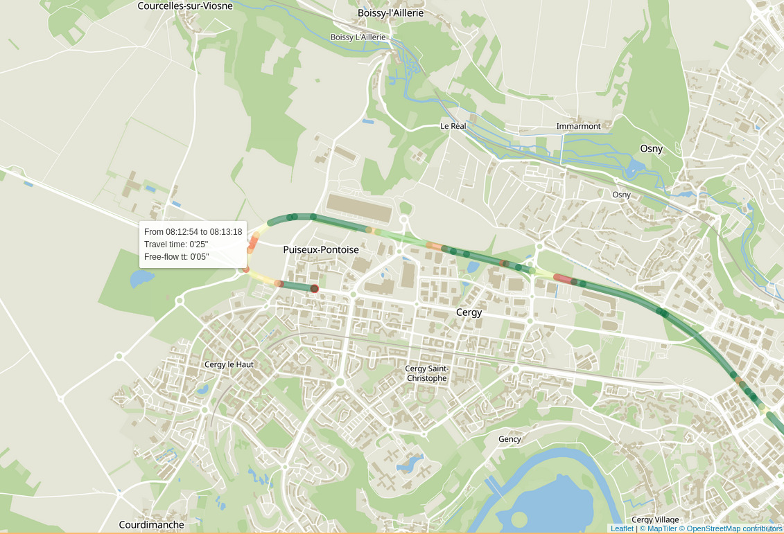
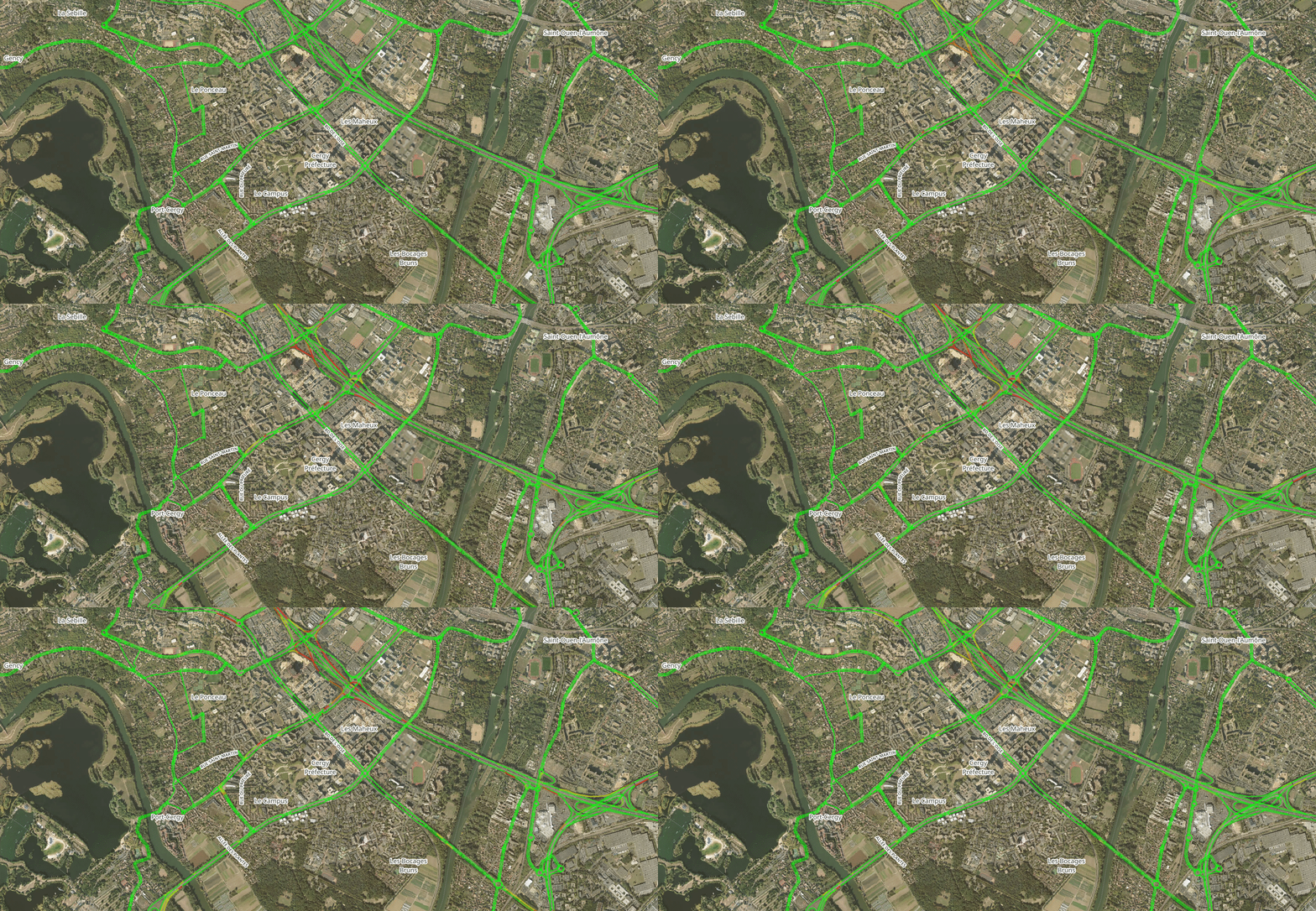
Congestion on each road
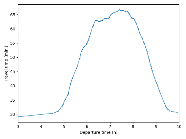
Origin-destination travel times

Other Transport Simulators

Macroscopic 4-step models:
- MODUS (DRIEAT)
- Antonin (Île-de-France Mobilités)
- GLOBAL (RATP)
Agent-based models:
- MATSim
- SimMobility (MIT)
- Emme (INRO)
- Visum (PTV)

Application: Île-de-France

Introduction

What? First large-scale application of Metropolis v2, on Île-de-France
Goal? Show the capabilities of Metropolis v2 (in particular, for calibration)
Scope? Trips by car, morning peak hour

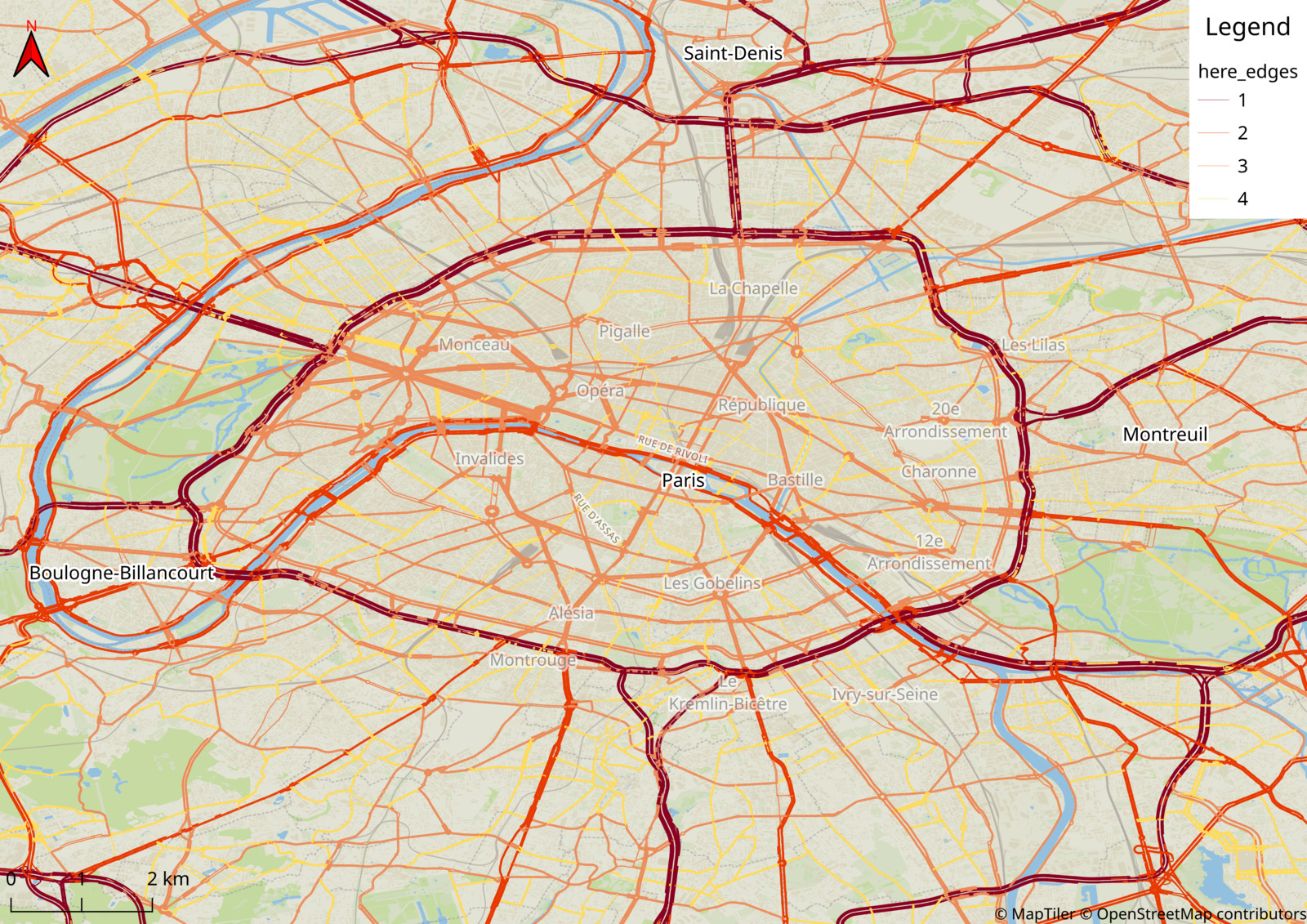
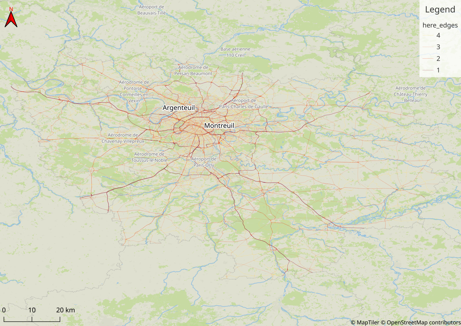
Input: Road network

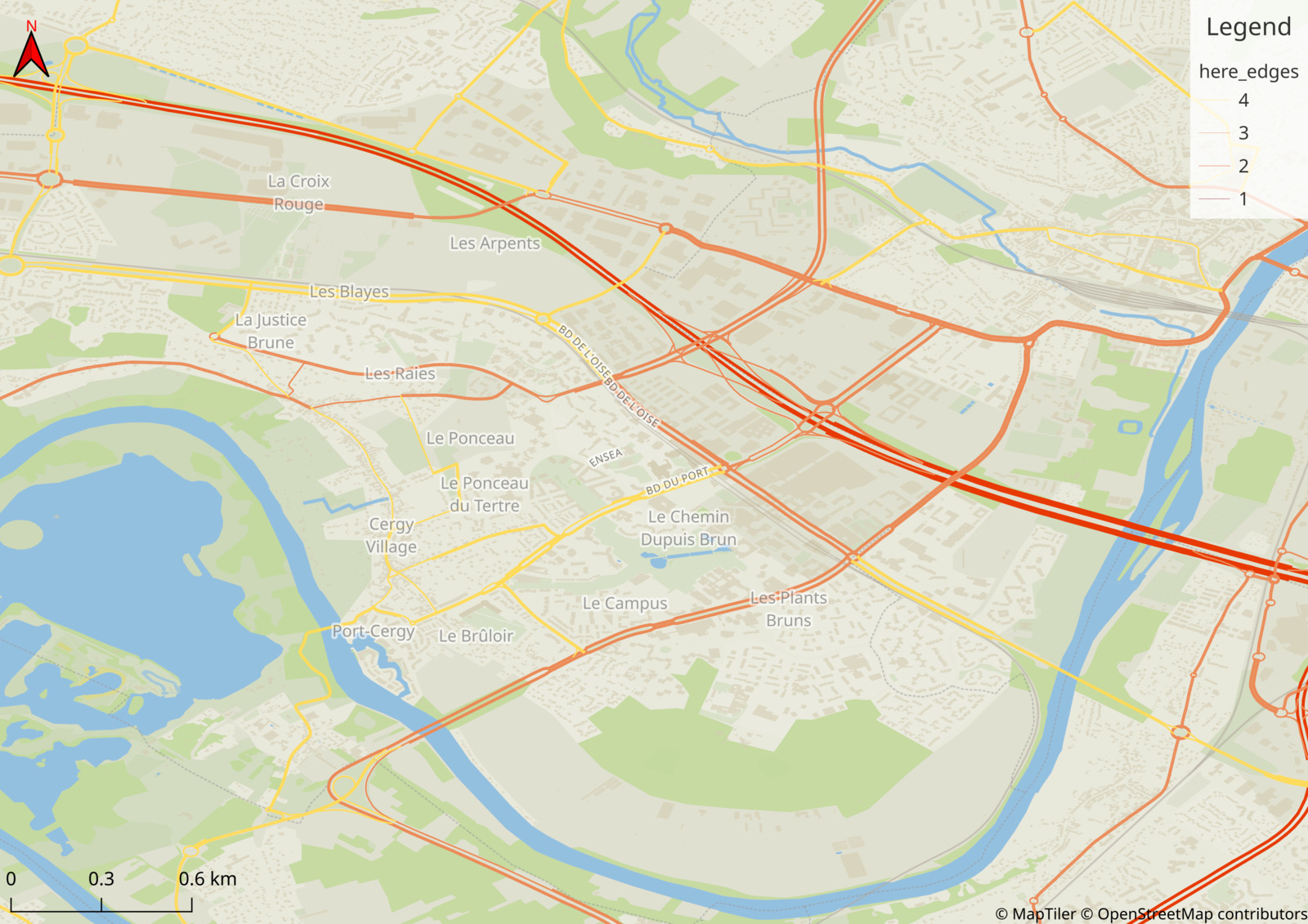
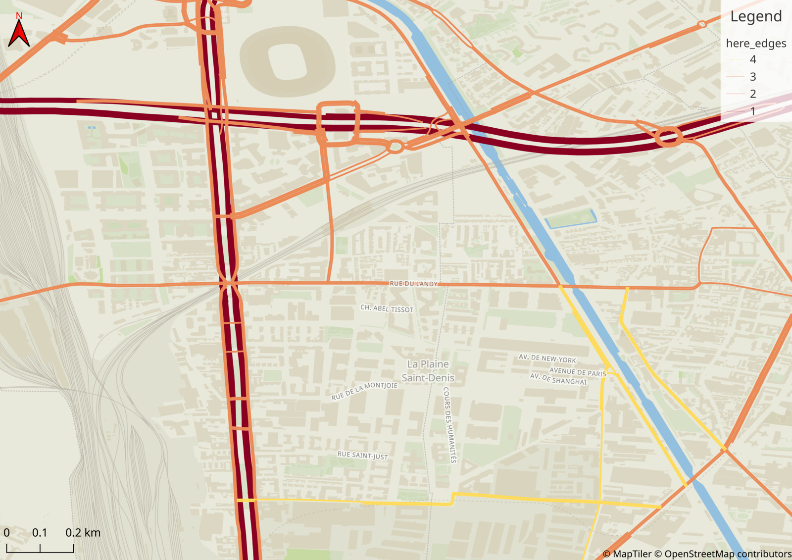
Source: HERE
Roads with functional class 1 to 4 are selected (i.e., less important roads are removed)
177 152 nodes and 308 027 edges

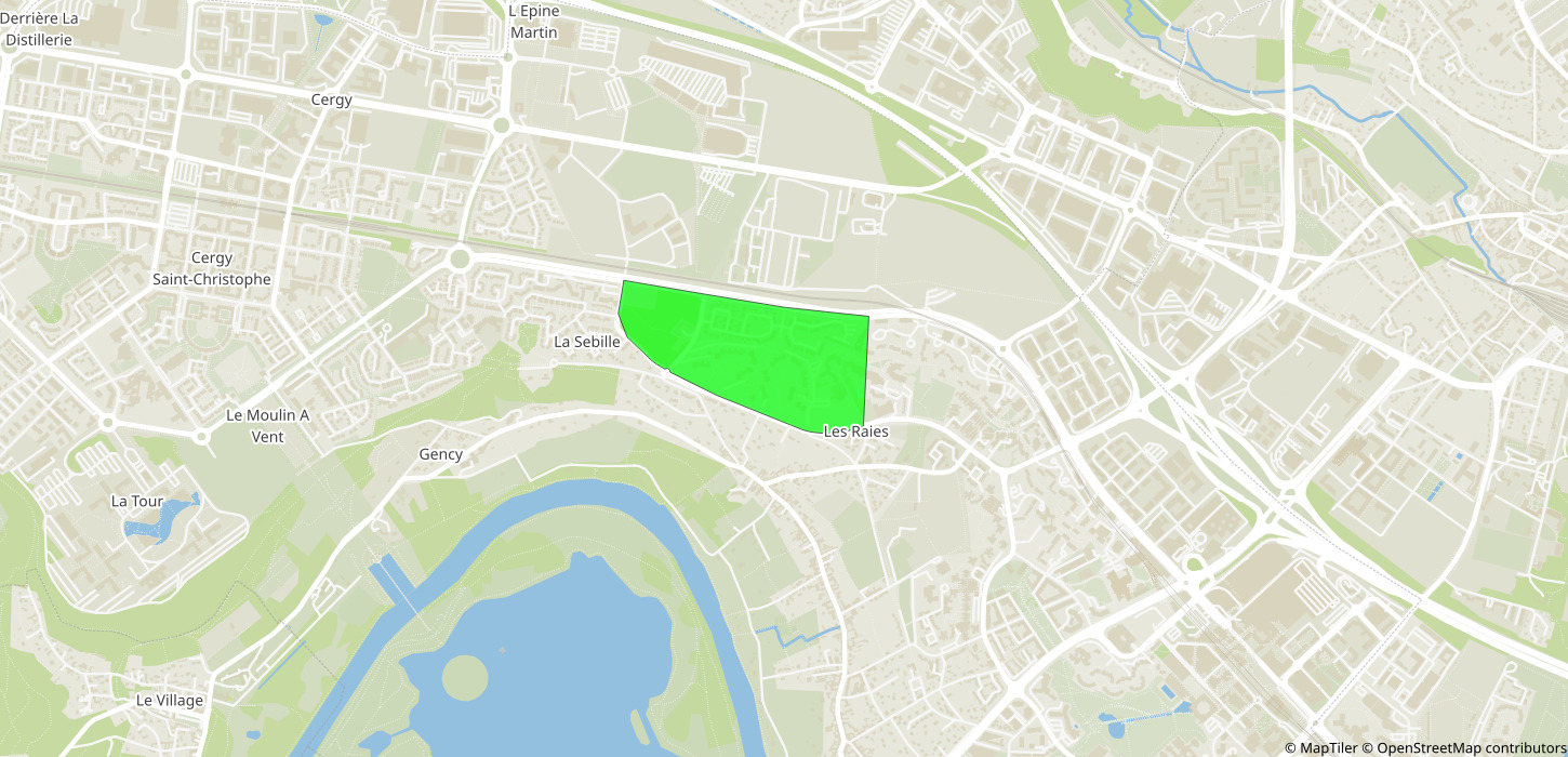
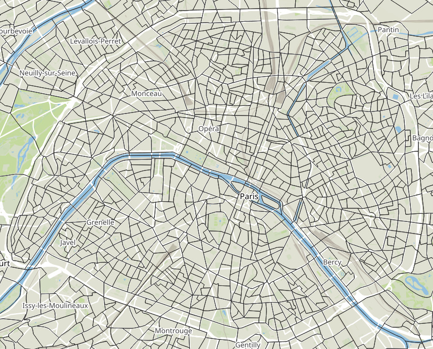
Input: Zones

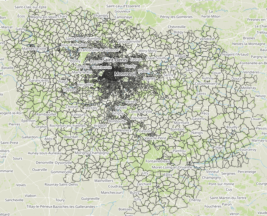
The origin and destination of the trips is aggregated at the IRIS zone level
IRIS zones: created by INSEE, homogeneous buildings, population of around 2000 inhabitants

5265 IRIS zones in Île-de-France

992 IRIS zones in Paris

Zone area: 2.292 km2 (mean), 0.330 km2 (median)

Input: Connectors

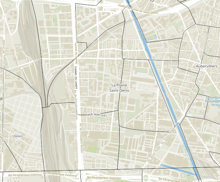
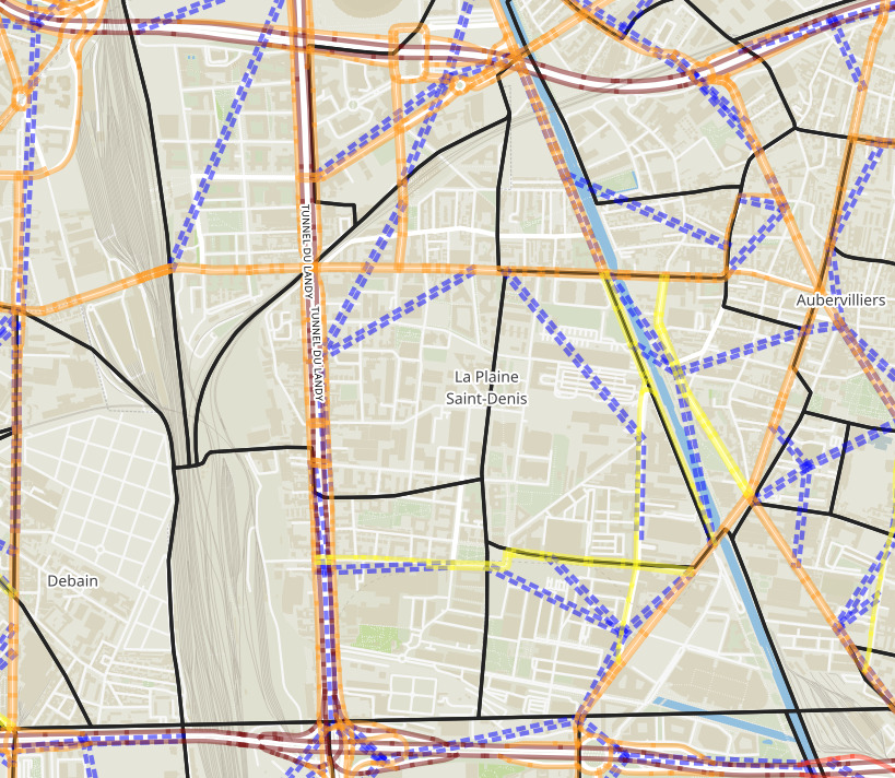
Zones are connected to the road network through virtual roads, called connectors
A virtual node can have up to 4 connectors, in each direction (incoming and outgoing)
Connectors have 1 lane and a speed limit of 30 km/h
Average travel time on connectors is 76 seconds

Data: Population

Trips are generated by combining many sources (INSEE census, travel survey, buildings data, etc.)
Filters: trips by car, from 3AM to 10AM, different origin and destination
Preference parameters chosen from the literature
185 572 trips are simulated (simulation is scaled down to 10 %)

Hörl, S. and Balac, M., 2021. Synthetic population and travel demand for Paris and Île-de-France based on open and publicly available data. Transportation Research Part C: Emerging Technologies, 130, p.103291.

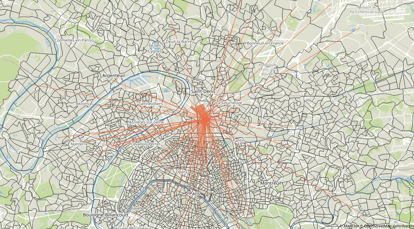
Trips to IRIS 930661102 (Saint-Denis - Plaine 02)

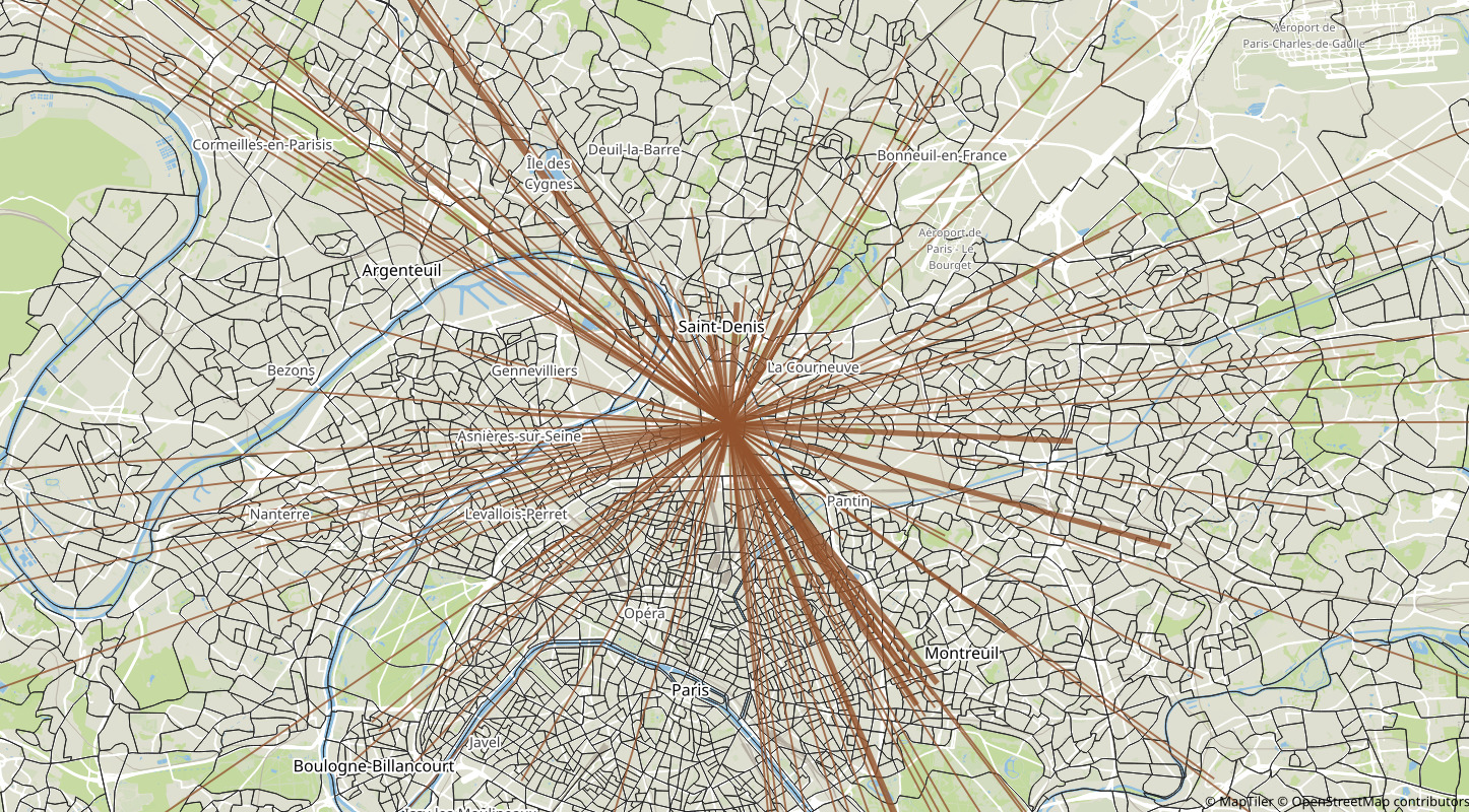
Trips from IRIS 930661102 (Saint-Denis - Plaine 02)

Running Metropolis

Network skims computation: computes origin-destination travel times given edges' travel times
Pre-day model: computes agents' mode, departure time and route choice
Within-day model: simulates congestion
Day-to-day model: computes expected edges' travel times given observed congestion

Network skims computation

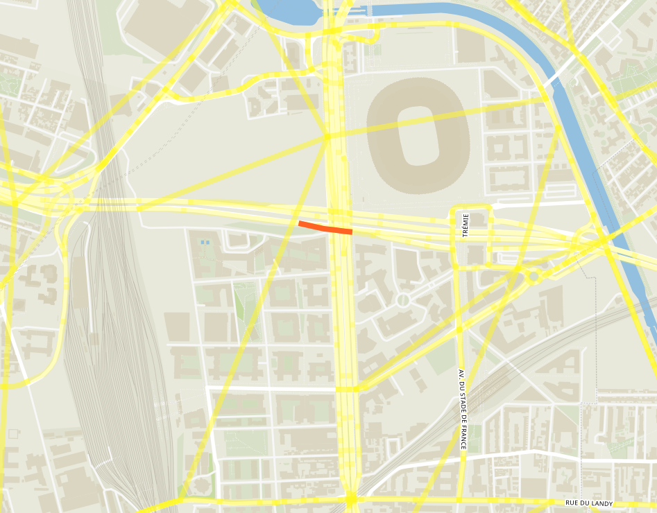
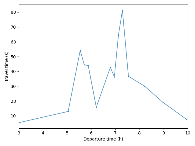
Input: edges' travel-time functions
Algorithm: Time-dependent contraction hierarchies
Output: origin-destination travel-time functions

Geisberger, R. and Sanders, P., 2010. Engineering time-dependent many-to-many shortest paths computation. In 10th Workshop on Algorithmic Approaches for Transportation Modelling, Optimization, and Systems (ATMOS'10). Schloss Dagstuhl-Leibniz-Zentrum fuer Informatik.

Pre-Day Model

Input: agents' characteristics and origin-destination travel-time functions
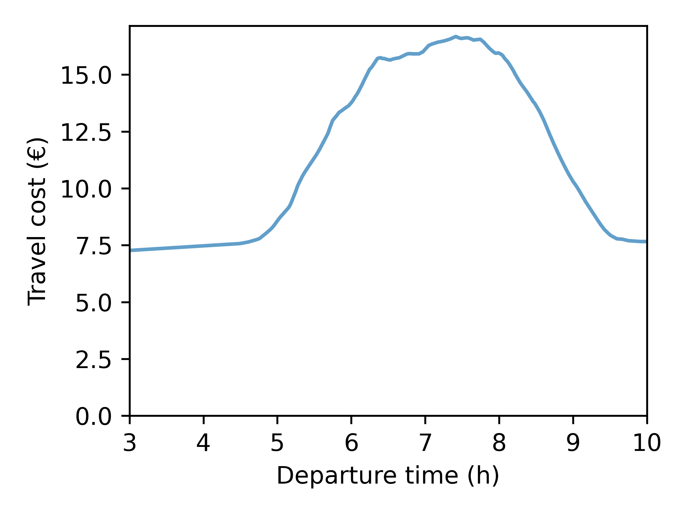
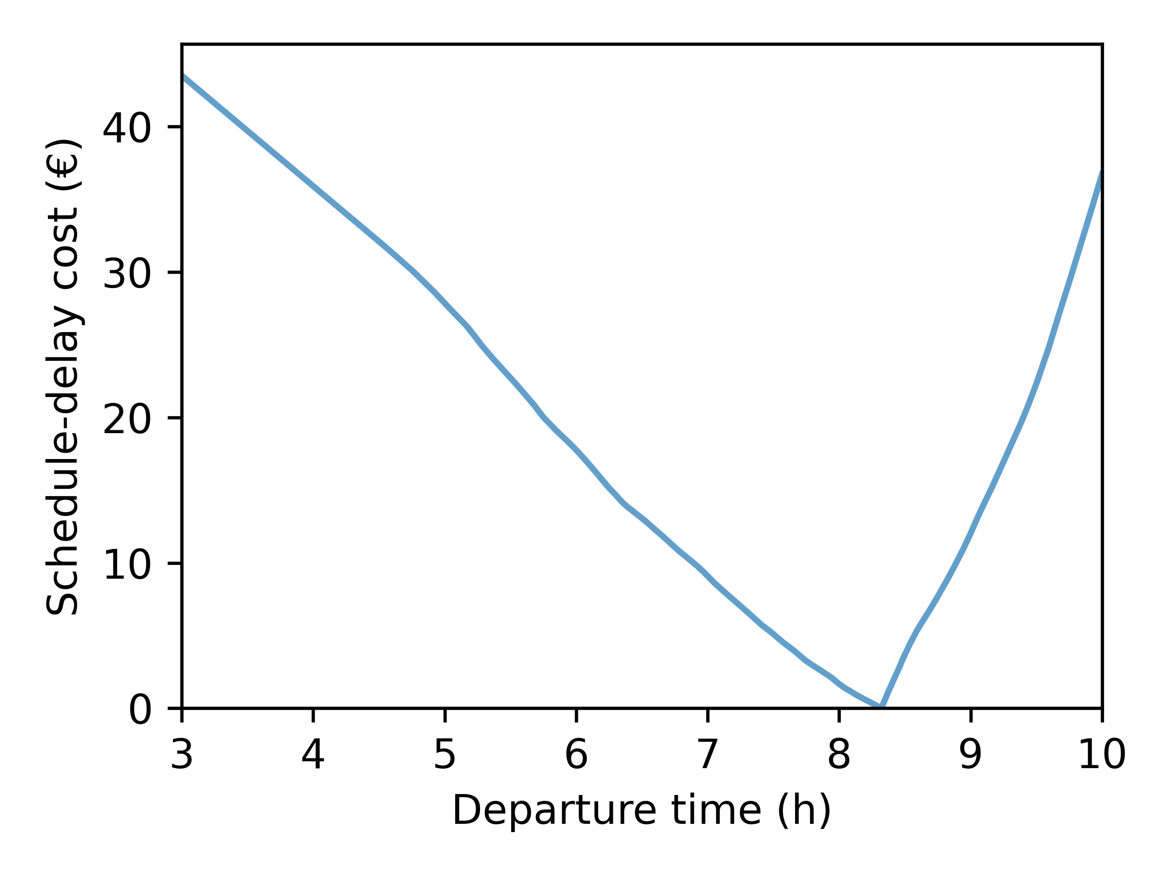
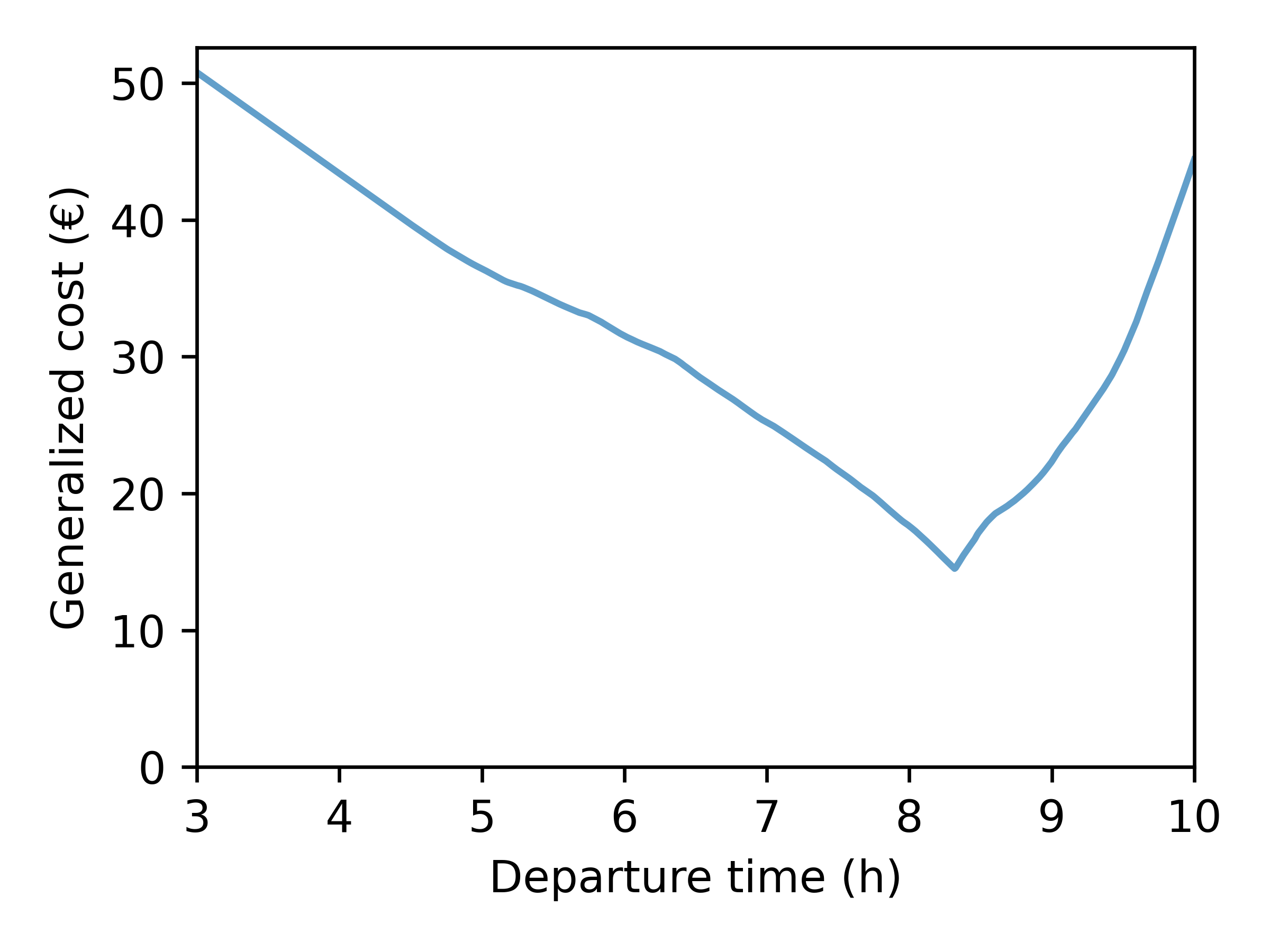
Step 1: Compute generalized costs
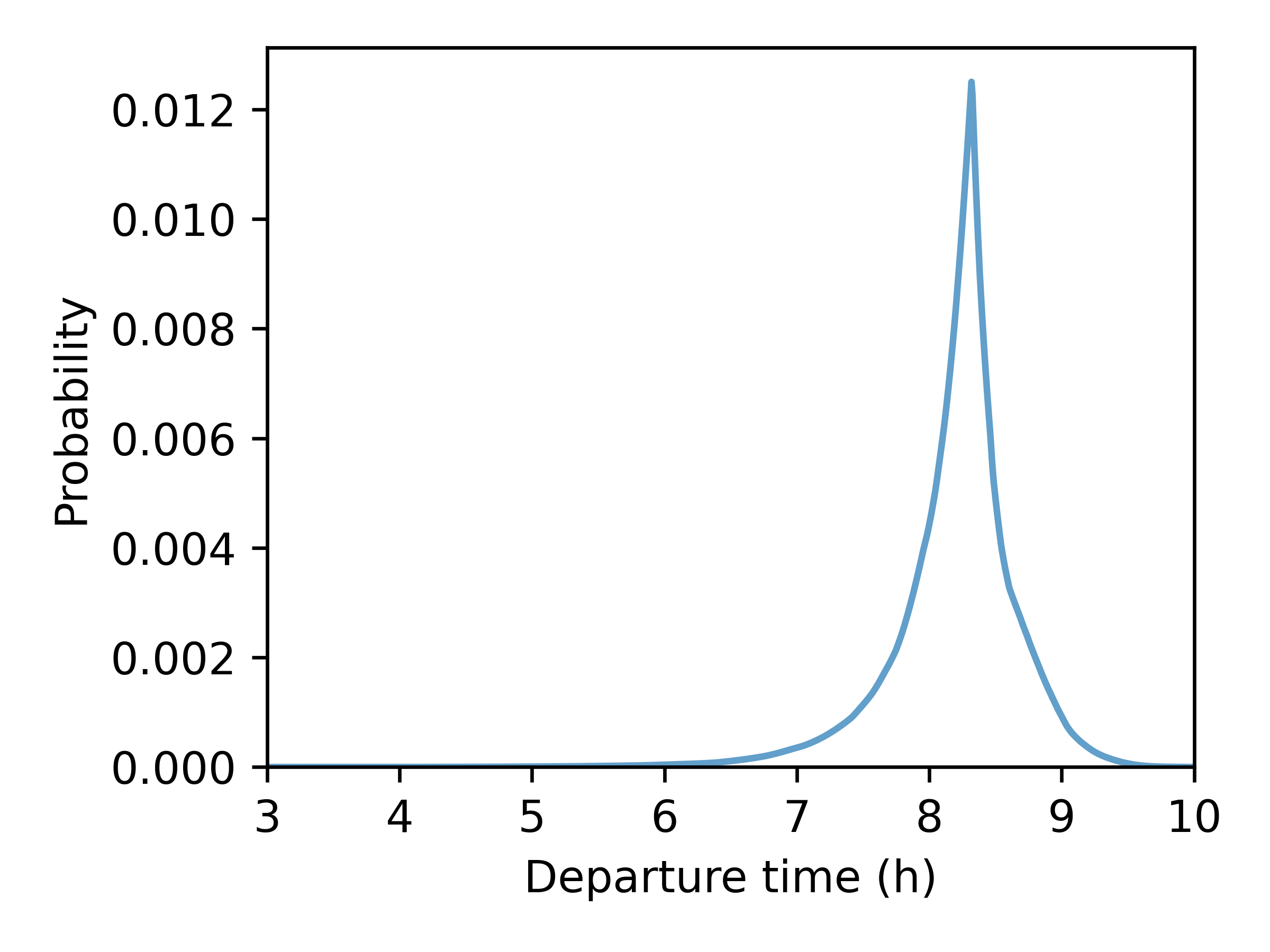
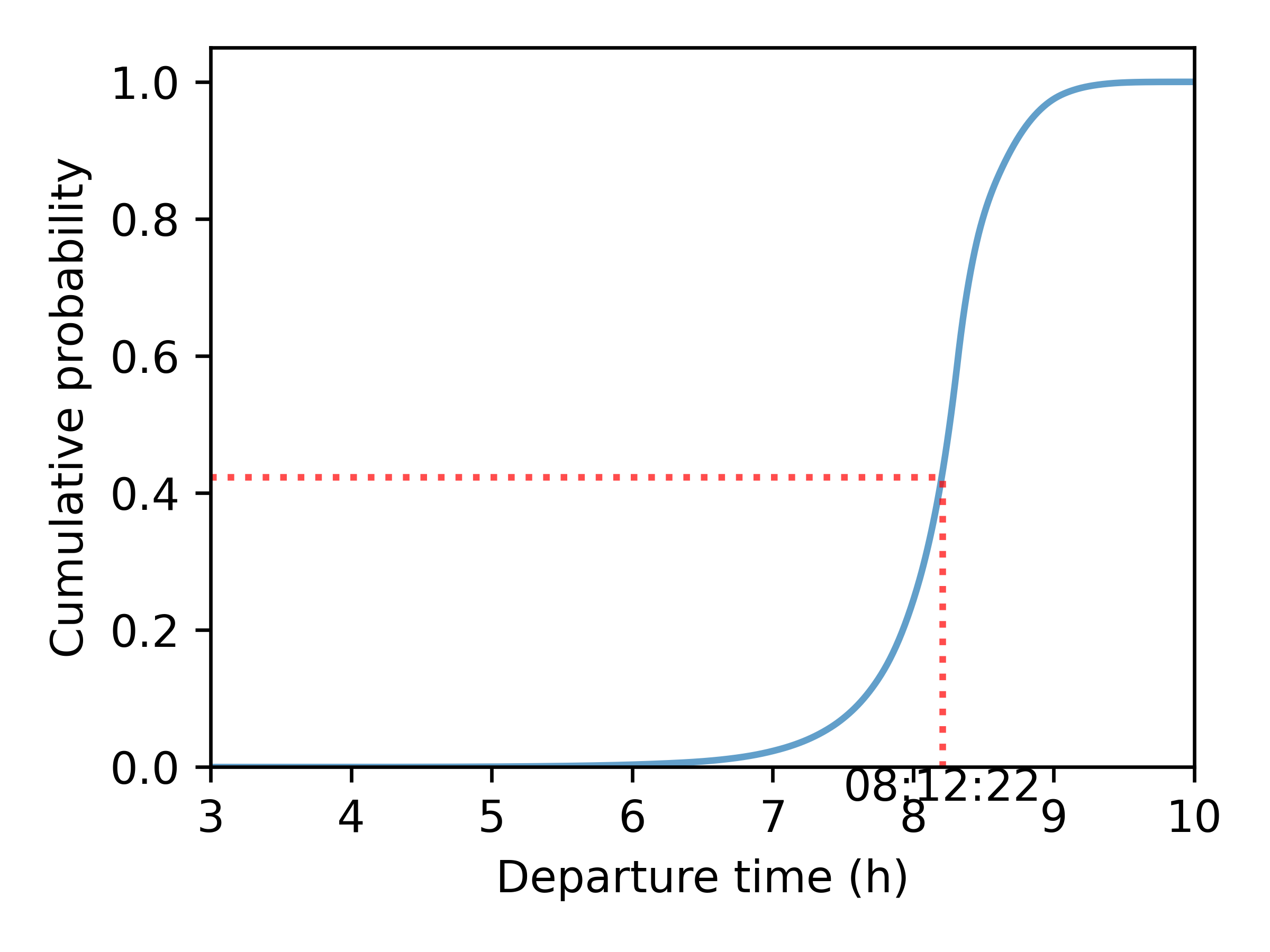
Step 2: Find chosen departure time (Continuous Logit Model)
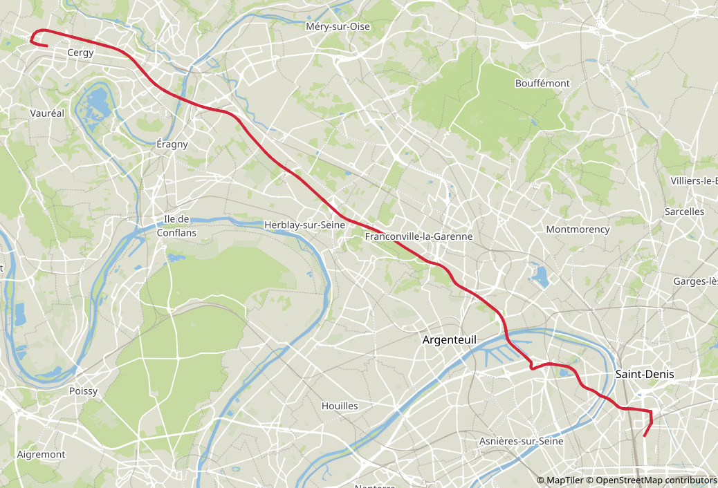
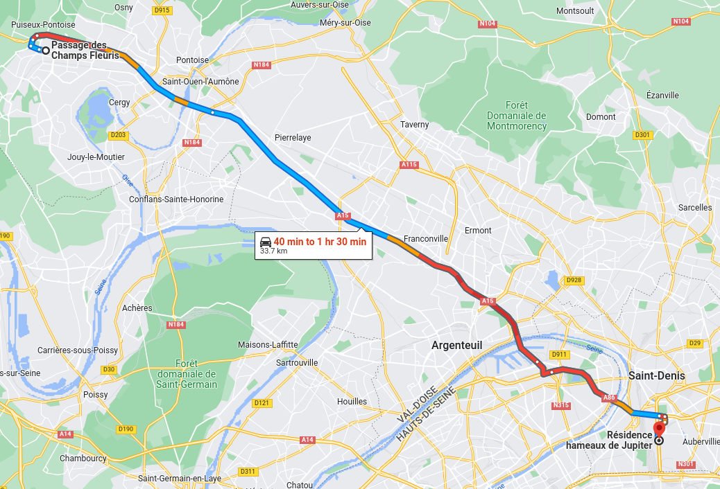
Step 3: Find chosen route (fastest path given departure time)

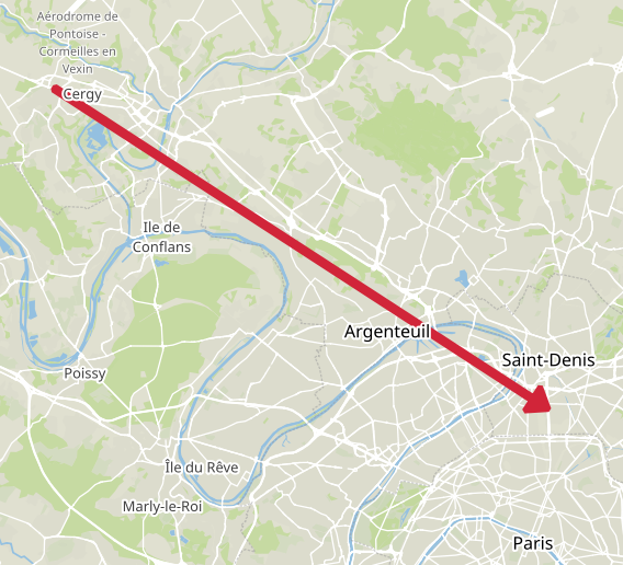
Origin: 951270127 (Cergy – Justice-Heuruelles)
Destination: 930661102 (Saint-Denis – Plaine 02)
Value of time: 15 € / h
Early penalty: 7.5 € / h
Late penalty: 30 € / h
Desired arrival time: 09:15

\[ c(t_d, t_a) = \underbrace{\alpha \cdot (t_a - t_d)}_{\text{travel cost}} + \underbrace{\beta \cdot [t^* - t_a]_+ + \gamma \cdot [t_a - t^*]_+}_{\text{schedule-delay cost}} \]

Within-Day Model

Input: Chosen mode, departure time and route of each agent
Agents' actions are simulated in a chronological order
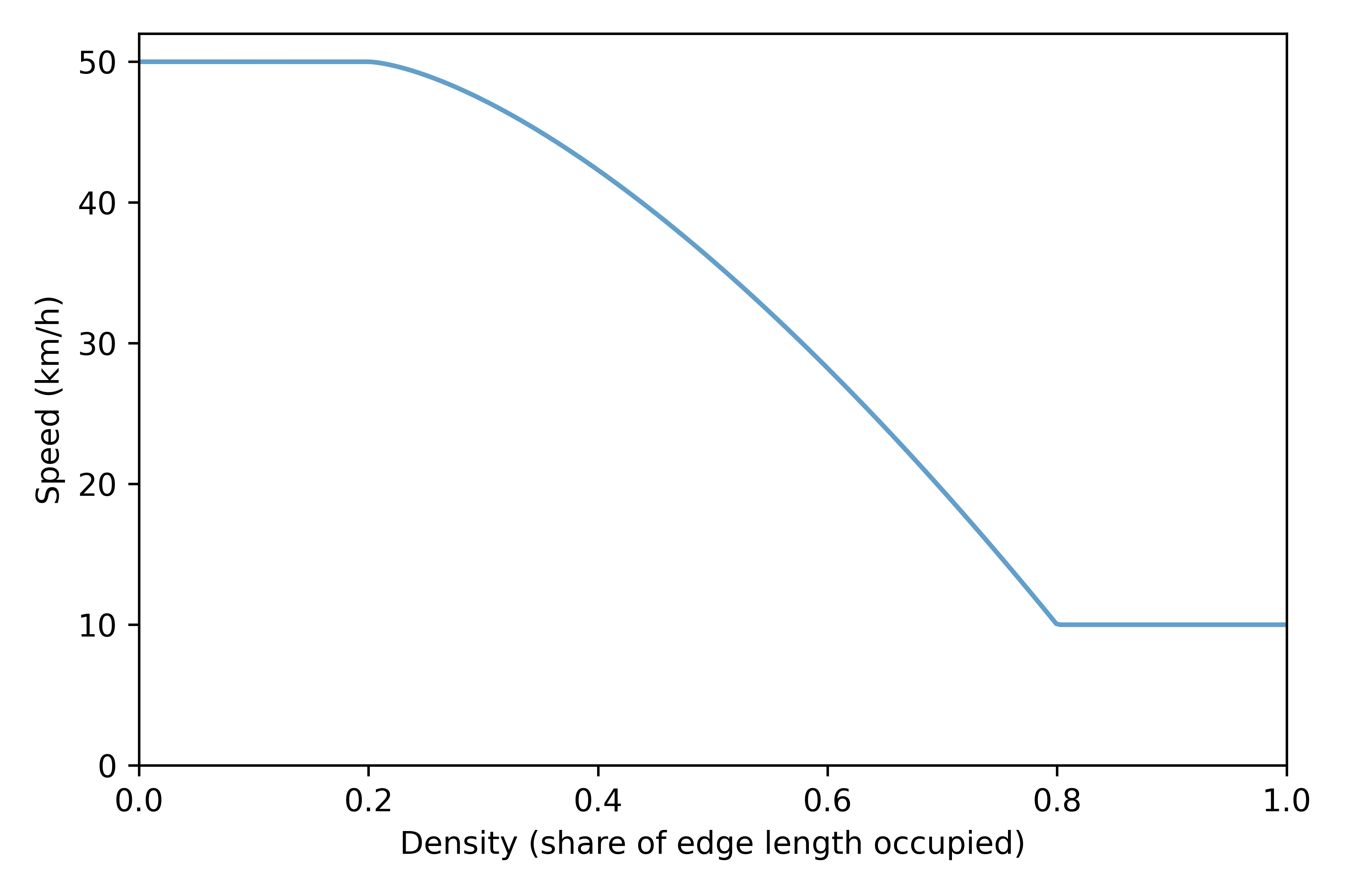
Congestion is simulated with speed-density functions and bottlenecks
Output: Edges' travel-time functions

Time	Event
03:00:03	Agent 91735 leaves origin through edge 317770
03:00:11	Agent 111697 leaves origin through edge 161026
03:00:11	Agent 157315 leaves origin through edge 99613
03:00:18	Agent 134340 leaves origin through edge 68763
03:00:21	Agent 152934 leaves origin through edge 137501
03:00:31	Agent 43475 leaves origin through edge 16265
03:00:34	Agent 111697 takes edge 161020

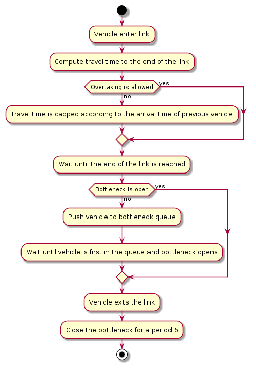
Day-to-Day Model

Input: Expected and simulated edges' travel-time functions
Learning process based on Markov decision processes
Stop the simulation if a stopping criteria is reached (e.g., maximum number of iterations, difference between expected and simulated travel times)
Output: Expected edges' travel-time functions for next iteration

\[ {tt}^e_{\tau + 1} = \lambda \cdot {tt}^e_{\tau} + (1 - \lambda) \cdot {tt}^s_{\tau} \]

Calibration (1/2)

Travel time penalties at intersections are calibrated to match travel time distribution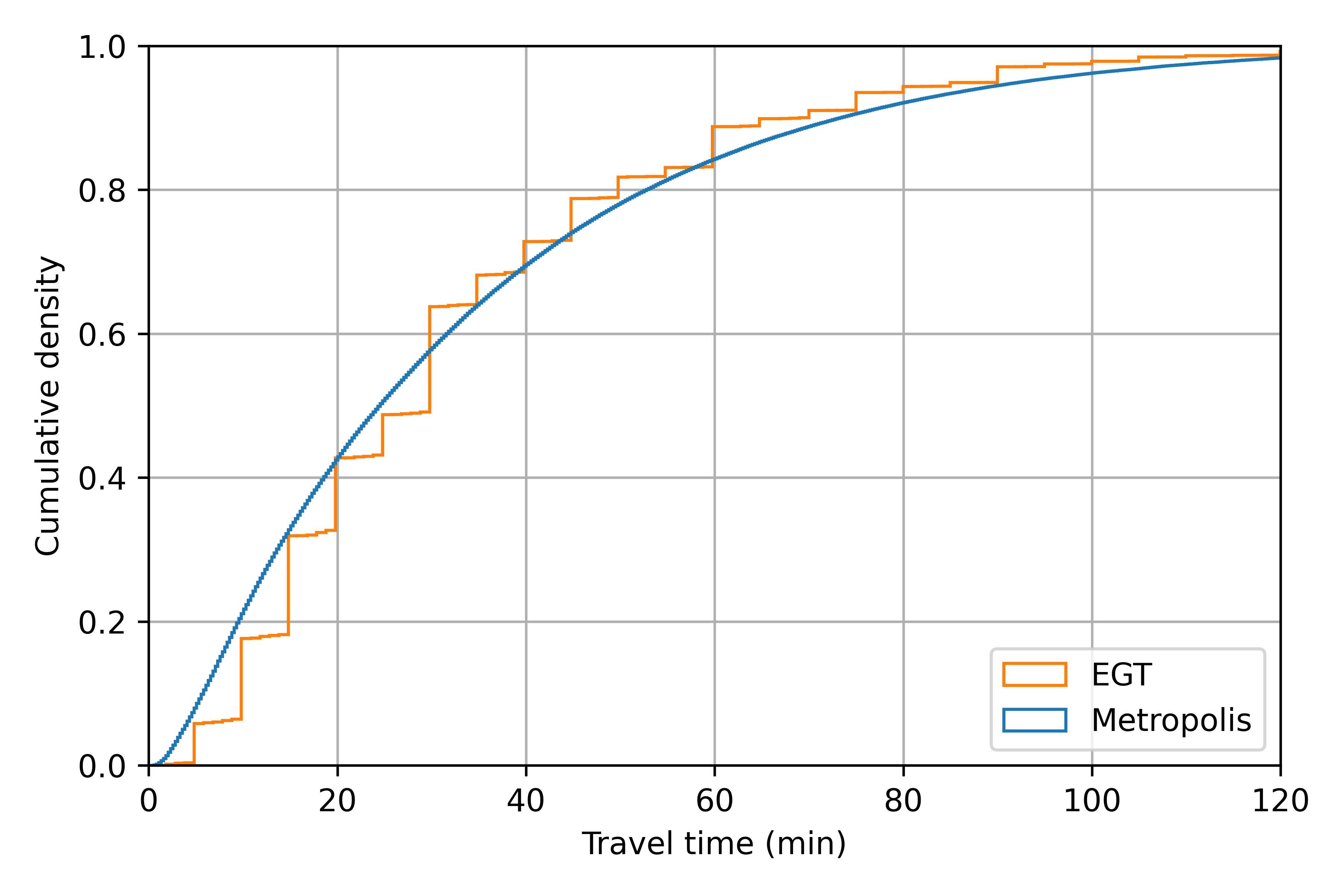

Calibration (2/2)

Distribution of desired arrival times is calibrated to match arrival time distribution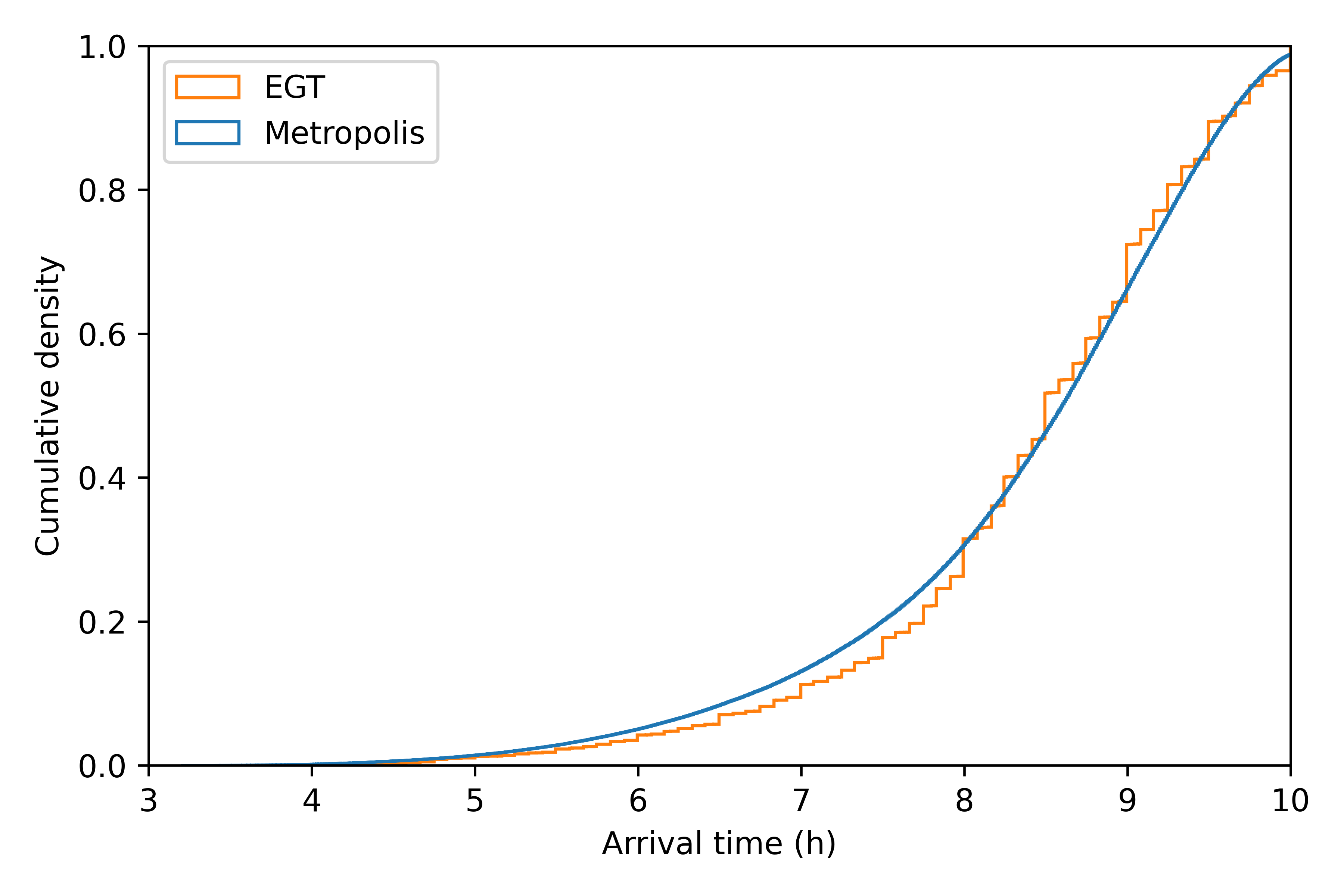

Aggregate Results

All values are averages over agents.

Value	Metropolis	EGT
Departure time	07:48:07	07:50:21
Arrival time	08:21:24	08:23:49
Travel time	00:33:17	00:33:28
Free-flow travel time	00:22:37
Distance	14.803 km
Departure-time shift*	2 seconds
Surplus	15.55 €
Free-flow surplus	18.56 €

Cost of congestion: 3.01 €

* Absolute difference between departure time from one iteration to another

Disaggregate Results: Agents' Trip

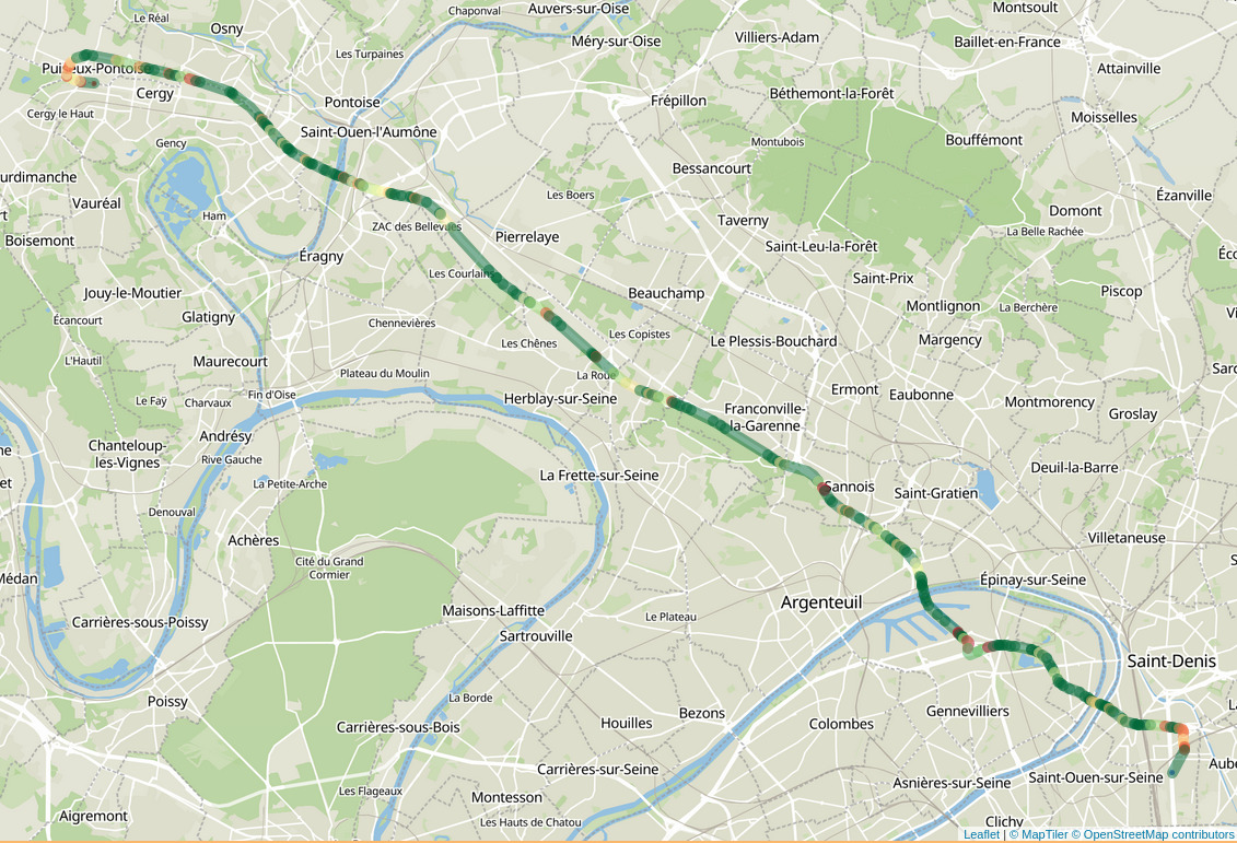
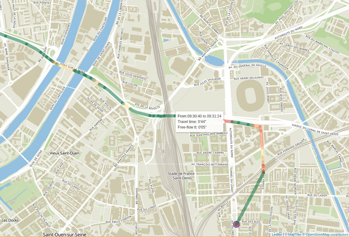
Id: 11484148
Departure time: 08:10:06
Arrival time: 09:35:31
Travel time: 01:25:25
Generalized cost: 30.52 €

Disaggregate Results: Road Congestion

Disaggregate Results: Origin-Destination Travel Time Functions

Example Policy

Basic policy scenario: 20 % of agents are removed randomly
Interpretation: shift to public transit or carpooling; increasing telecommute

Value	Baseline	Policy	Change
Departure time	07:48:07	07:53:18	+ 5'11''
Arrival time	08:21:24	08:22:57	+ 1'33''
Travel time	00:33:17	00:29:39	- 3'38''
Distance	14.803 km	14.900 km	+ 97m
Surplus	15.55 €	16.59 €	+ 1.04 €

Conclusion and Future Works

Public Transit

Differences compared to private transport:
- Number of transfers, walking time, in-vehicle congestion and reliability have to be considered, in addition to travel time
- Departure-time choice is a discrete choice (as opposed to continuous)
Objectives for next year:
- Departure-time and route (= lines) choice
- Generalized cost includes walking time, waiting time, mode-specific times (bus, subway, etc.) and in-vehicle congestion
- Sitting is modeled explicitly

Future improvements

Road maintenance (Ravi Seshadri)
Automatic computation of air pollution (Romuald le Frioux)
Ride-sharing (Samarth Ghoslya)

Thank you for your attention