Metropolis
Basic Principle
- Metropolis is an iterative model
- At each iteration, four models are run successively (network skims computation, pre-day model, within-day model and day-to-day model)
- The simulation stops when a convergence criteria is met or when the maximum number of iterations is reached

Input of the Model
The input of Metropolis can be divided in three main categories:- Road network
- Population (list of agents and their characteristics)
- Simulation parameters
- Id: 11484148
- Purpose: Home to work
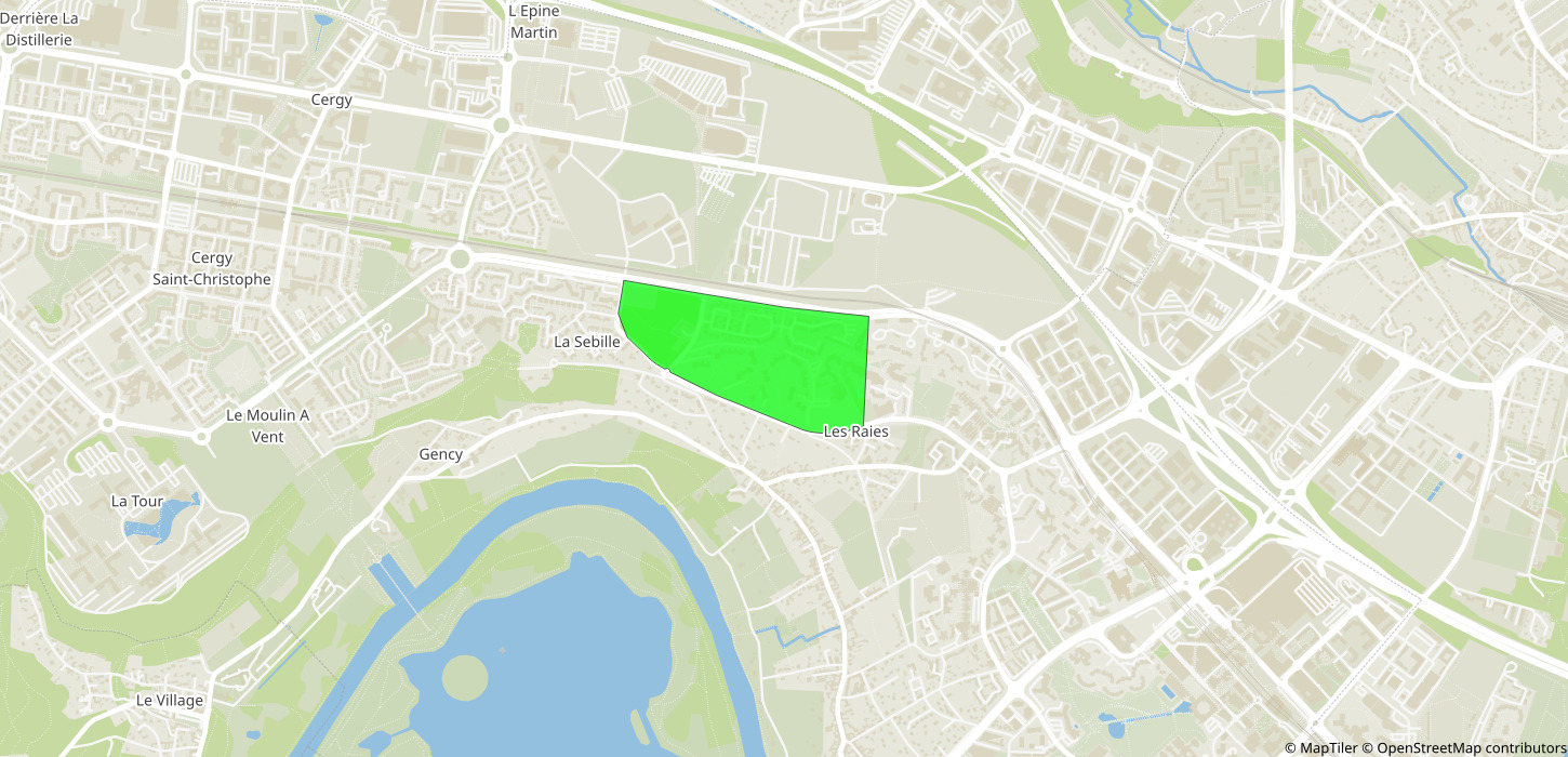
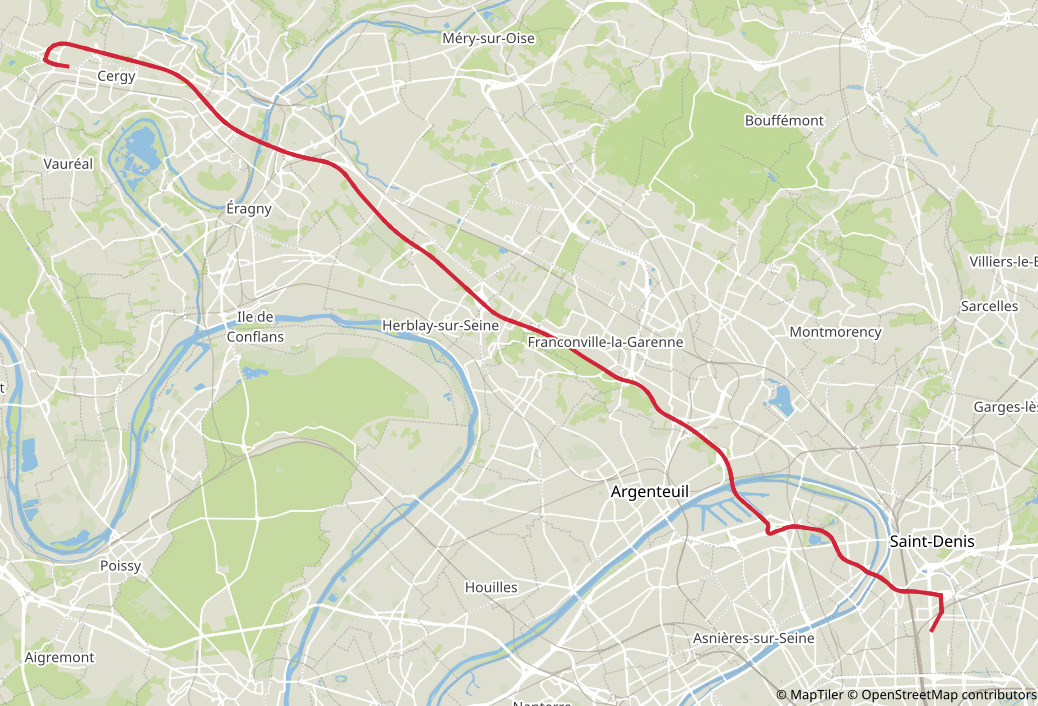
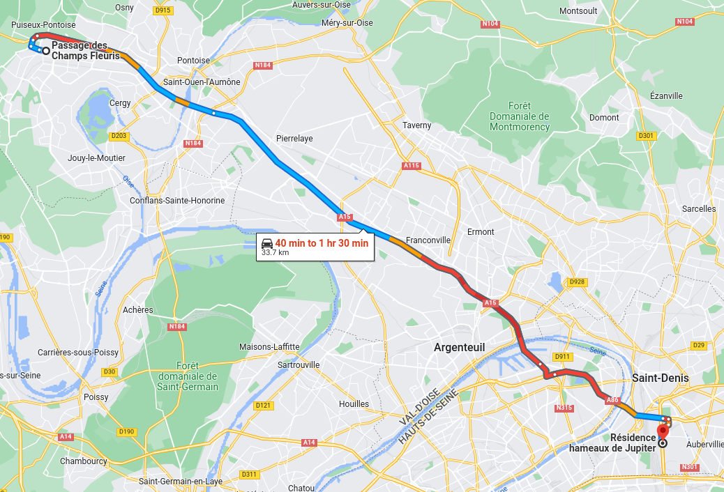
- Origin: 951270127 (Cergy – Justice-Heuruelles)
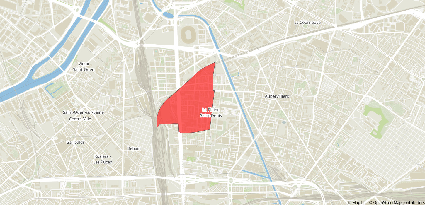
- Destination: 930661102 (Saint-Denis – Plaine 02)
- Age: 39
- Sex: male
- Employed: Yes
- Socioprofessional class: 3 (executive)
- Driving license: Yes
- Monthly household income: 3369 euros
Other Transport Simulators
-
Macroscopic 4-step models:
- MODUS (DRIEAT)
- Antonin (Île-de-France Mobilités)
- GLOBAL (RATP)
-
Agent-based models:
- MATSim
- SimMobility (MIT)
- Emme (INRO)
- Visum (PTV)
Transport Simulators
- TransCAD (Caliper)
- Emme-3 (INRO)
- Visum / Vissim (PTV)
- DYNASMART-P (McTrans)
- Mezzo (KTH Royal Institute of Technology)
- SimMobility (MIT)
- MATSim (VSP TU-Berlin / IVT ETH Zurich)
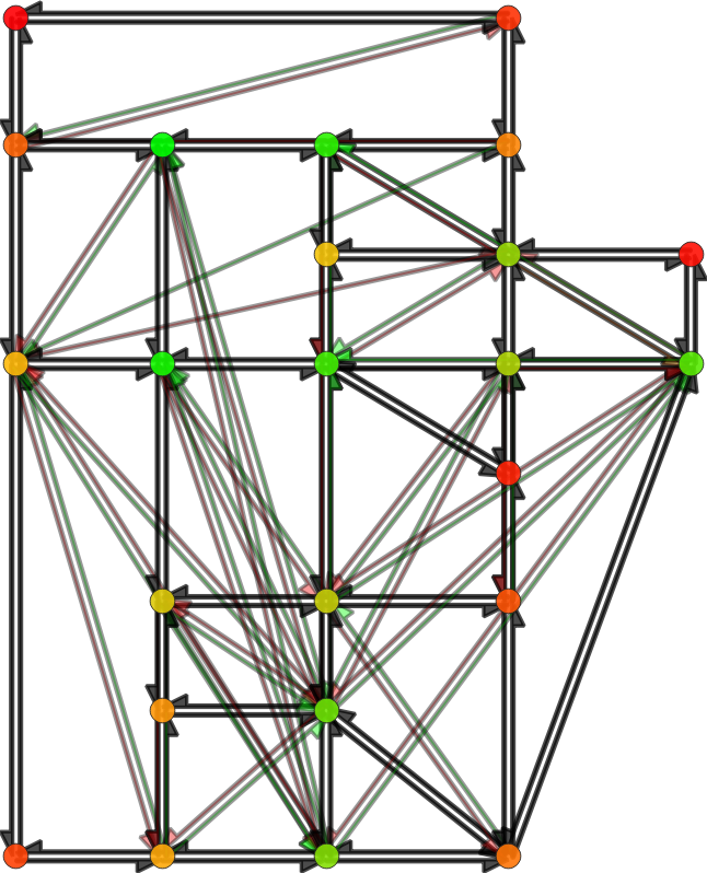
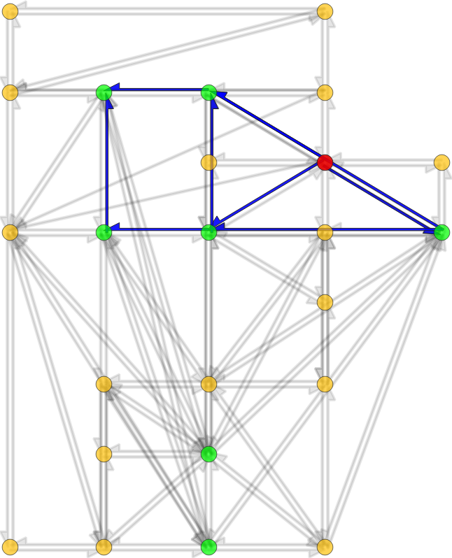
Network skims computation
- Input: time-dependent travel-time function for each road of the road-network graph
- Step 1: compute a time-dependent Hierarchy Overlay of the graph
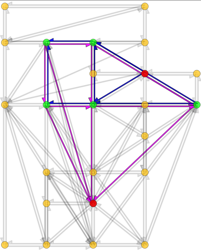
- Step 2: compute search spaces for each origin and destination node
- Step 3: compute profile queries for each origin-destination pair
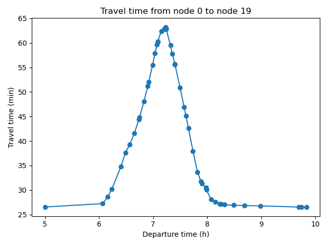
- Output: time-dependent travel-time function for each origin-destination pair (with at least one trip)
Geisberger, R. and Sanders, P., 2010. Engineering time-dependent
many-to-many shortest paths computation. In
10th Workshop on Algorithmic Approaches for Transportation
Modelling, Optimization, and Systems (ATMOS'10). Schloss Dagstuhl-Leibniz-Zentrum fuer Informatik.
Pre-Day Model
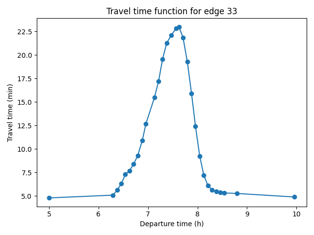
- Input: time-dependent travel-time function for each origin-destination pair
- Departure-time choice: choose the departure time of the agent, given the travel-time function, the schedule-utility and travel-utility functions and the mode (continuous Logit model)
- Route choice: choose the route that minimizes the travel time of the agent for the departure time chosen
- Mode choice: choose the mode of the agent, given the expected utility for each mode available (Logit model, deterministic model or any other choice model)
- Output: mode, departure-time and route chosen by each agent
Note. For some modes, there is no departure-time and route choice.
Day-to-Day Model
- Input: expected and simulated time-dependent travel-time function for each road
- Compute the expected travel-time functions for next iteration given the expected and simulated travel-time functions of current iteration, using a Markov process (e.g., exponential process with weight $\lambda$ for simulated values)
- Stop the simulation if a stopping criteria is reached (e.g., maximum number of iterations, EXPECT threshold, departure-time shift threshold)
- Output: expected time-dependent travel-time function for each road
Running Metropolis
Basic Principle
Running the Metropolis simulator can be summarized by these three steps:- Write the input JSON files
- Run the simulator in a terminal
- Read and analyze the output JSON files
Input Files
Metropolis requires 3 input JSON files:- Road-network: list of edges with their characteristics, list of vehicle types with their characteristics
- Agent file: list of the agents with their characteristics (including modes available)
- Simulation parameters
Units
- Time: number of seconds since midnight (10AM is 36 000)
- Travel time: number of seconds
- Length: meters
- Speed: meters per second (50 km/h is 50 ÷ 3.6 m/s)
- Value of time: utility unit (e.g., €, $ or an abstract unit) per second
- Flow: vehicle length (in meters) per second
Road Network JSON File
Example Road Network JSON File
{
"graph": {
"edges": [
[
0,
1,
{
"base_speed": 10.0,
"length": 10.0,
"constant_travel_time": 1.0,
"bottleneck_flow": 1.0,
"lanes": 2,
"speed_density": {
"type": "FreeFlow"
},
"overtaking": true
}
],
[
1,
2,
{
"base_speed": 20.0,
"length": 10.0,
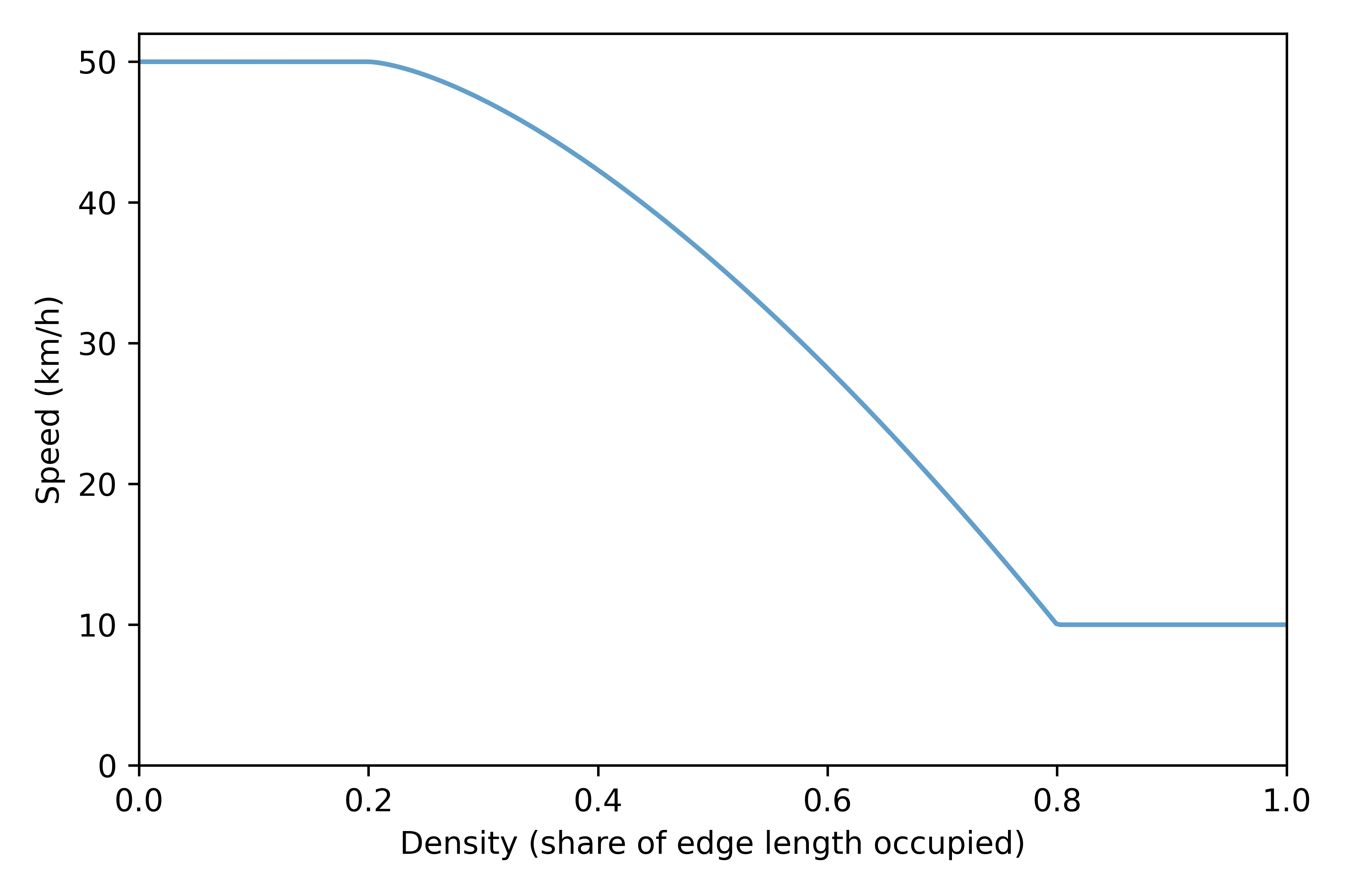
"speed_density": {
"type": "ThreeRegimes",
"value": {
"beta": 1.1,
"jam_density": 0.2,
"jam_speed": 2.0,
"min_density": 0.8
}
}
}
]
]
},
"vehicles": [
{
"headway": 10.0,
"pce": 1.0
},
{
"headway": 30.0,
"pce": 5.0,
"speed_function": {
"type": "Piecewise",
"value": [
[
0.0,
0.0
],
[
25.0,
25.0
],
[
100.0,
25.0
]
]
},
"restricted_edges": [
1
]
}
]
}
Agent JSON File
Example Agent JSON File
[
  {
    "id": 1,
    "mode_choice": {
      "type": "Logit",
      "value": {
        "u": 0.5,
        "mu": 1.0
      }
    },
    "modes": [
      {
        "type": "Trip",
        "value": {
          "legs": [
            {
              "class": {
                "type": "Road",
                "value": {
                  "origin": 0,
                  "destination": 1,
                  "vehicle": 0
                }
              },
              "stopping_time": 600.0,
              "travel_utility": {
                "type": "Polynomial",
                "value": {
                  "a": 1.0,
                  "b": -0.003
                }
              },
              "schedule_utility": {
                "type": "None"
              }
            },
            {
              "class": {
                "type": "Virtual",
                "value": 300.0
              },
              "travel_utility": {
                "type": "Polynomial",
                "value": {
                  "b": -0.003
                }
              }
            }
          ],
          "departure_time_model": {
            "type": "ContinuousChoice",
            "value": {
              "period": [
                0.0,
                200.0
              ],
              "choice_model": {
                "type": "Logit",
                "value": {
                  "u": 0.5,
                  "mu": 1.0
                }
              }
            }
          },
          "origin_schedule_utility": {
            "type": "None"
          },
          "destination_schedule_utility": {
            "type": "AlphaBetaGamma",
            "value": {
              "t_star_low": 30.0,
              "t_star_high": 30.0,
              "beta": 1.0,
              "gamma": 4.0
            }
          },
          "pre_compute_route": true
        }
      },
      {
        "type": "Trip",
        "value": {
          "legs": [
            {
              "class": {
                "type": "Virtual",
                "value": 900.0
              }
            }
          ],
          "departure_time_model": {
            "type": "Constant",
            "value": 50.0
          }
        }
      }
    ]
  }
]
Parameters JSON File
Example Parameters JSON File
{
  "period": [
    0.0,
    200.0
  ],
  "network": {
    "road_network": {
      "recording_interval": 50.0,
      "approximation_bound": 1.0,
      "spillback": true,
      "max_pending_duration": 20.0,
      "algorithm_type": "Best"
    }
  },
  "learning_model": {
    "type": "Exponential",
    "value": {
      "alpha": 0.99
    }
  },
  "init_iteration_counter": 1,
  "stopping_criteria": [
    {
      "type": "MaxIteration",
      "value": 2
    },
    {
      "type": "DepartureTime",
      "value": [
        0.01,
        100.0
      ]
    }
  ],
  "update_ratio": 1.0,
  "random_seed": 19960813,
  "nb_threads": 24
}
Running the Simulator
Output Files
Metropolis output 7 different file types:-
log.txt: text file with the log of the simulation -
report.html: HTML file with a summary table and graphs -
iteration{n}.json: JSON file with aggregate results, for each iteration -
running_time.json: JSON file with running times for the different parts of the simulator -
agent_results.json.zst: compressed JSON file with agent-specific results -
skim_results.json.zst: compressed JSON file with network skim results (i.e., OD pair travel times) -
weight_results.json.zst: compressed JSON file with network weight results (i.e., edges' travel times)
report.html
iteration{n}.json
agent_results.json
skim_results.json
weight_results.json
Application Example
Running a full-scale application of Metropolis can be done in 5 steps (there is a Python script for each step):- Pre-processing the road network (e.g., from OpenStreetMap data)
- Connecting the origin/destination zones to the road network through connectors
- Generating the population
- Filtering the trips from the population that should be simulated
- Writing the Metropolis input files
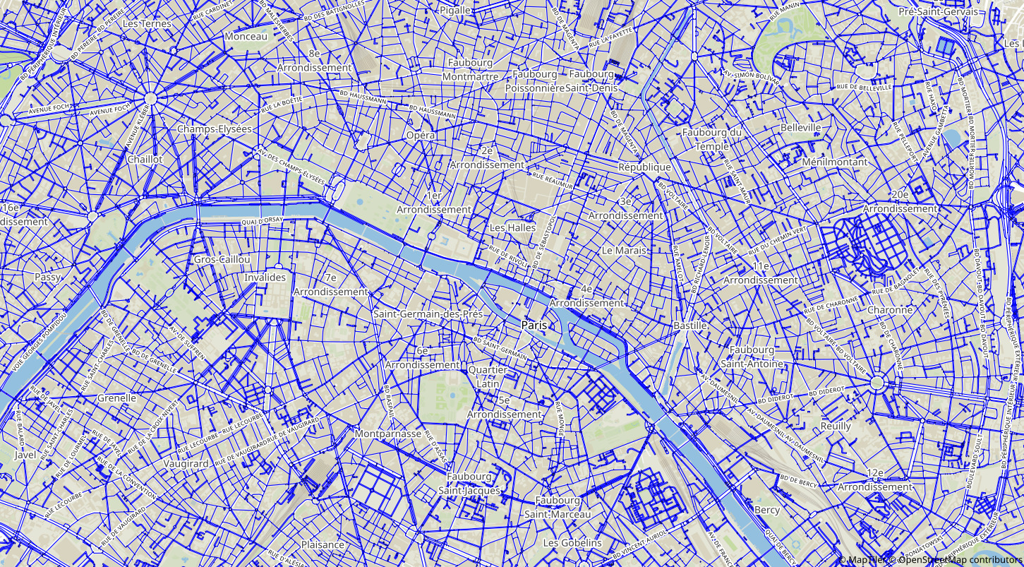
Pre-Processing the Road Network
- Compatible data sources: OpenStreetMap and HERE
- Country-level and region-level OpenStreetMap data can be downloaded from https://download.geofabrik.de
- Filters can be used to discard less relevant roads (e.g., roads tagged as "residential" in OpenStreetMap)
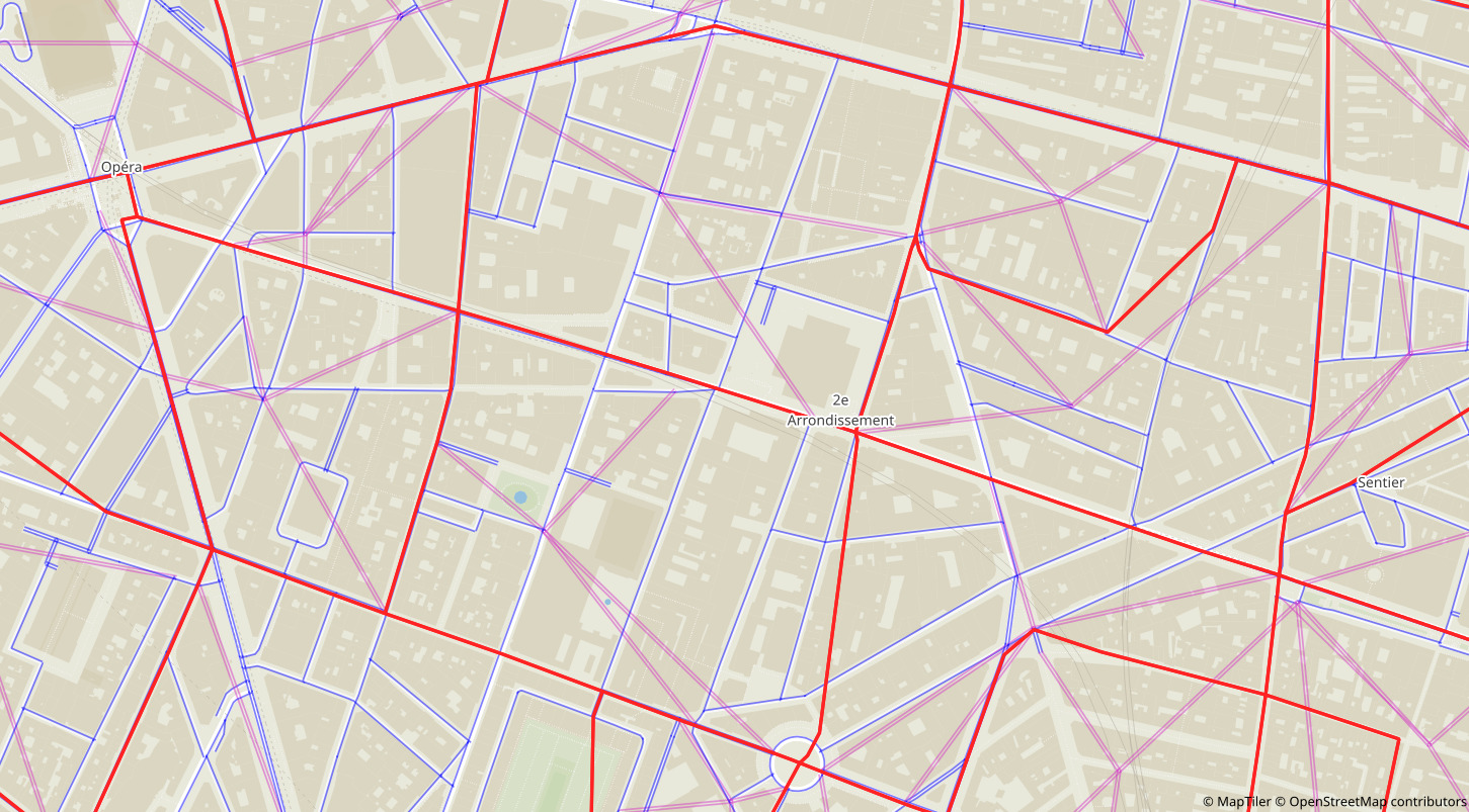
Creating Connectors
- Trips' departure/arrival points are aggregated at an origin/destination zone level
- In France, IRIS zones are a good compromise between accuracy and running time
- Virtual nodes are created to represent the departure/arrival points of the trips in a zone
- Connectors (virtual edges) are created to connect the virtual nodes to the road network
Generating and Filtering the Population
- A synthetic population can be created from Hörl and Balac (2021)'s methodology
- Python scripts to convert the output from Hörl and Balac (2021) to data compatible with Metropolis
- Filters: simulated period, modes
- Intra-zonal trips are removed
Hörl, S. and Balac, M., 2021. Synthetic population and travel demand for Paris and Île-de-France based on open and publicly available data. Transportation Research Part C: Emerging Technologies, 130, p.103291.
Writing Metropolis Input Files
- Python script to write the 3 Metropolis input JSON files from the output of the previous steps
-
Many parameters to choose and calibrate:
- Vehicle length and PCE
- Simulated period
- Individual preferences (alpha, beta, gamma, etc.)
- Edges' capacities
- Edges' constant travel times
Application: Île-de-France
Introduction
- What? First large-scale application of Metropolis v2, on Île-de-France
- Goal? Show the capabilities of Metropolis v2 (in particular, for calibration)
- Scope? Trips by car, morning peak hour
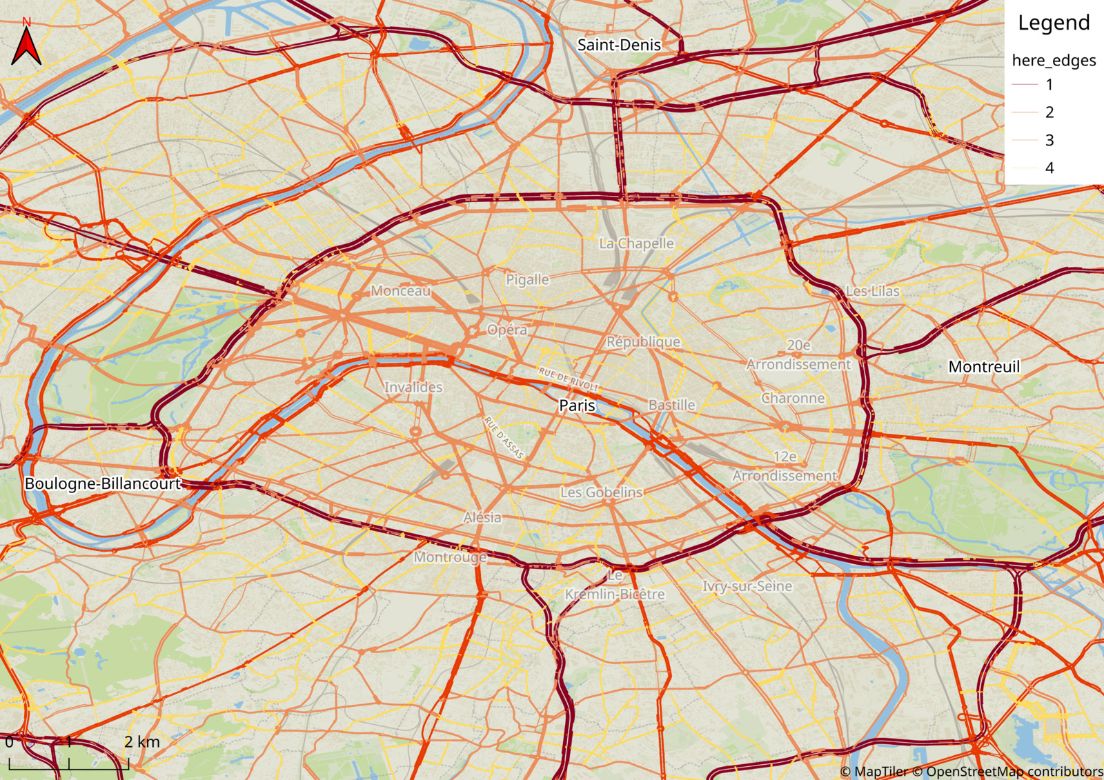
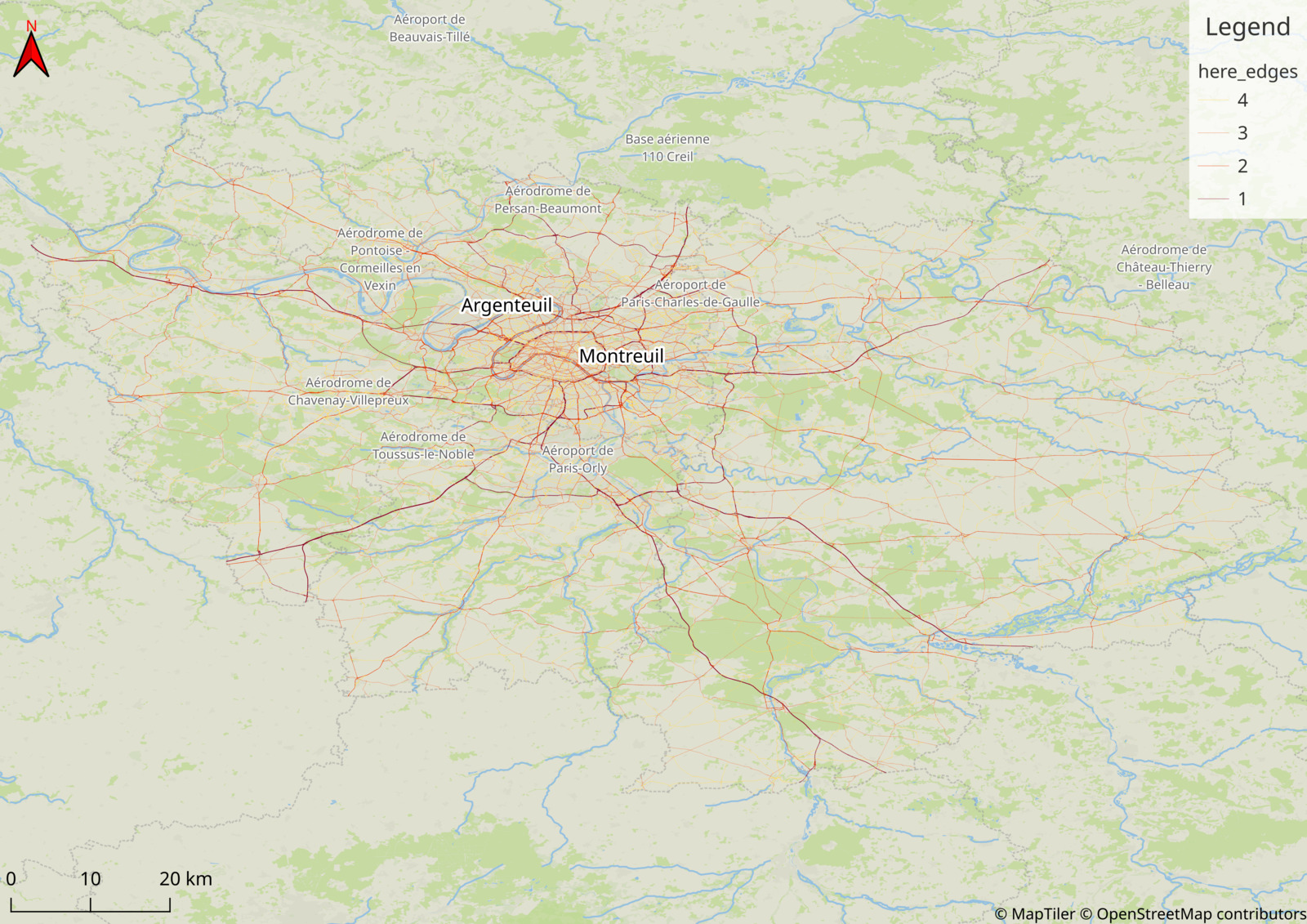
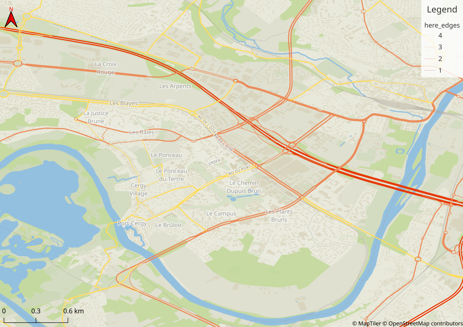
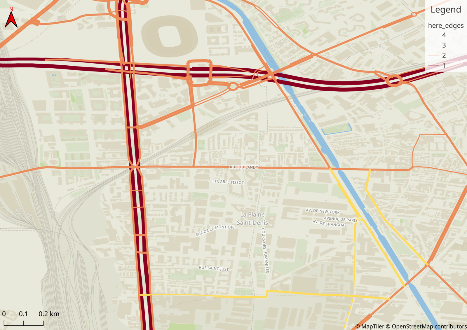
Input: Road network
- Source: HERE
- Roads with functional class 1 to 4 are selected (i.e., less important roads are removed)
- 177 152 nodes and 308 027 edges
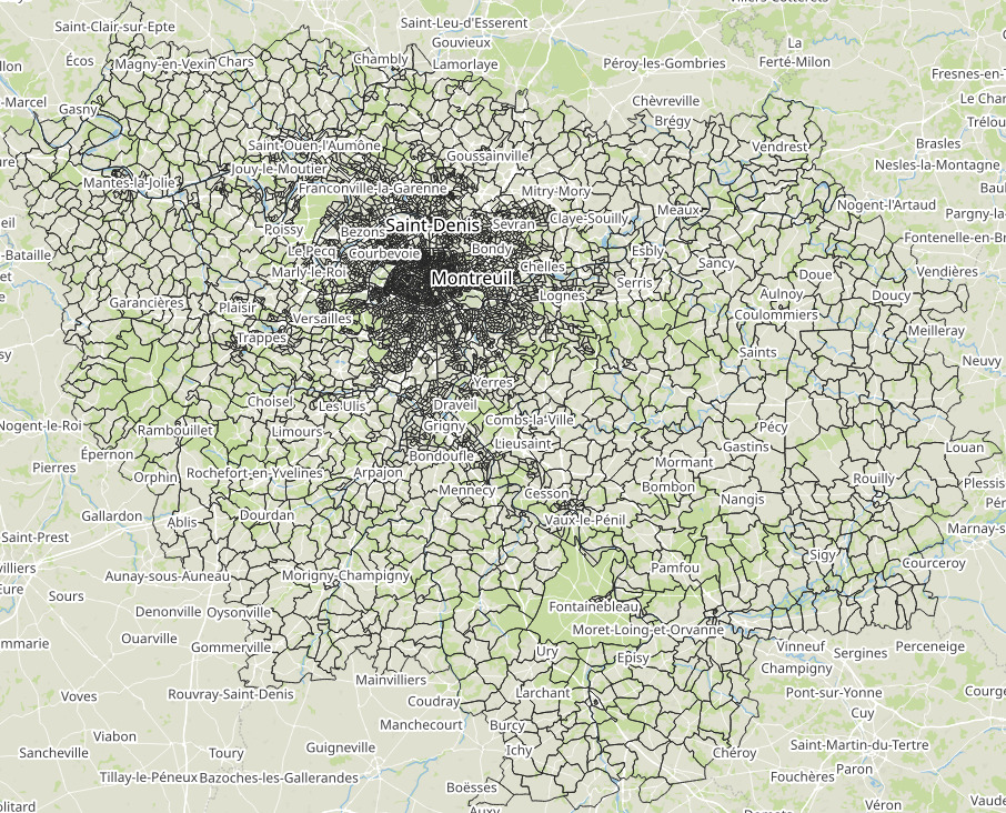
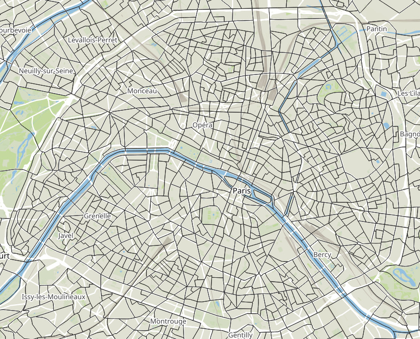
Input: Zones
- The origin and destination of the trips is aggregated at the IRIS zone level
- IRIS zones: created by INSEE, homogeneous buildings, population of around 2000 inhabitants
- 5265 IRIS zones in Île-de-France
- 992 IRIS zones in Paris
- Zone area: 2.292 km2 (mean), 0.330 km2 (median)
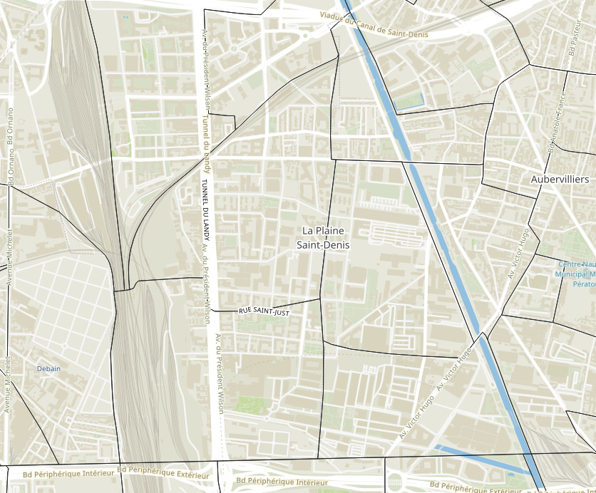
Input: Connectors
- Zones are connected to the road network through virtual roads, called connectors
- A virtual node can have up to 4 connectors, in each direction (incoming and outgoing)
- Connectors have 1 lane and a speed limit of 30 km/h
Data: Population
- Trips are generated by combining many sources (INSEE census, travel survey, buildings data, etc.)
- Filters: trips by car, from 3AM to 10AM, different origin and destination
- Preference parameters chosen from the literature
- 1 855 720 trips are simulated
Hörl, S. and Balac, M., 2021. Synthetic population and travel demand for Paris and Île-de-France based on open and publicly available data. *Transportation Research Part C: Emerging Technologies, 130*, p.103291.
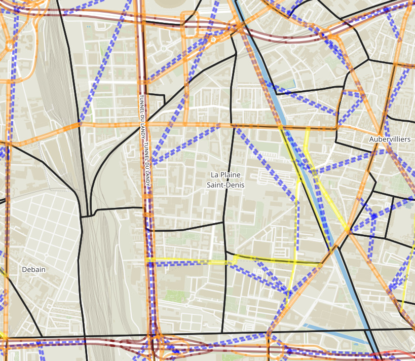
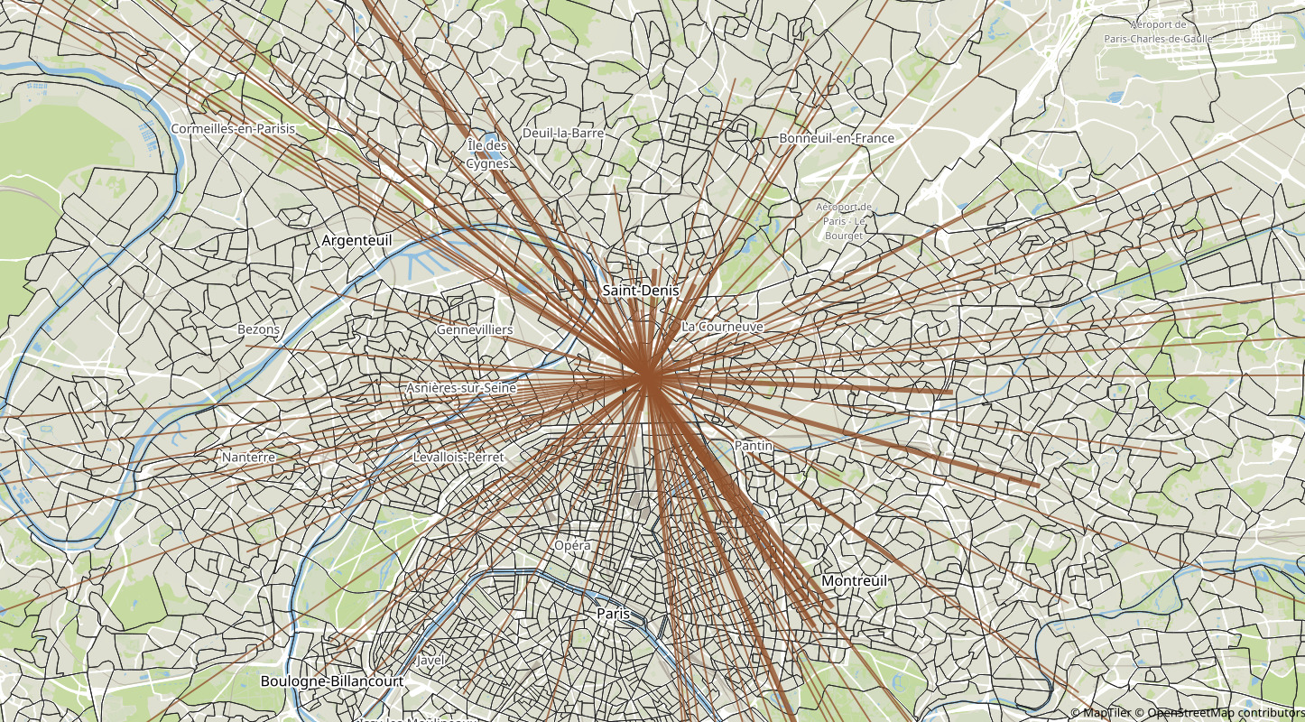
Trips to IRIS 930661102 (Saint-Denis - Plaine 02)
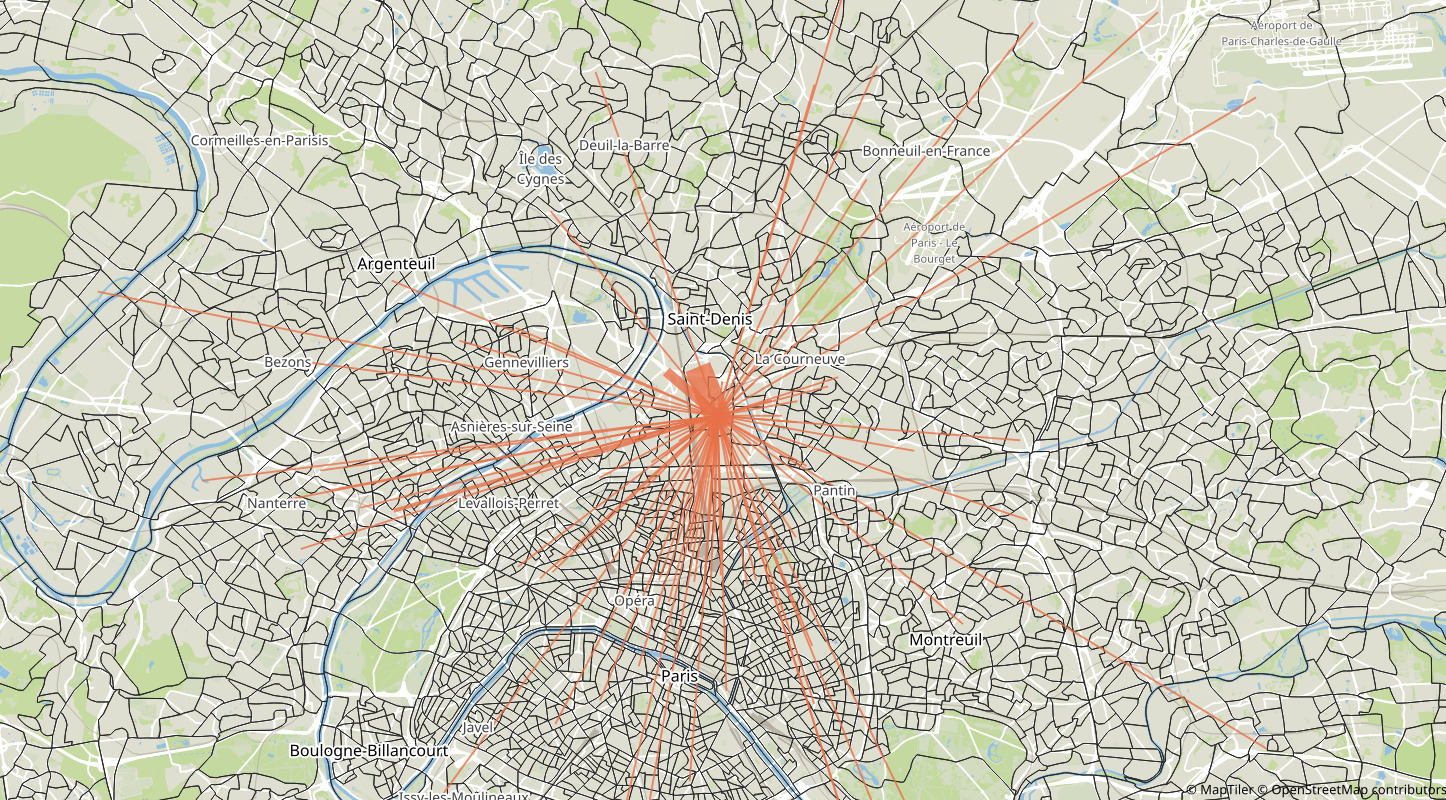
Trips from IRIS 930661102 (Saint-Denis - Plaine 02)
Running Metropolis
- Network skims computation: computes origin-destination travel times given edges' travel times
- Pre-day model: computes agents' mode, departure time and route choice
- Within-day model: simulates congestion
- Day-to-day model: computes expected edges' travel times given observed congestion
Network skims computation
- Input: edges' travel-time functions
- Algorithm: Time-dependent contraction hierarchies
- Output: origin-destination travel-time functions
Geisberger, R. and Sanders, P., 2010. Engineering time-dependent
many-to-many shortest paths computation. In
10th Workshop on Algorithmic Approaches for Transportation
Modelling, Optimization, and Systems (ATMOS'10). Schloss Dagstuhl-Leibniz-Zentrum fuer Informatik.
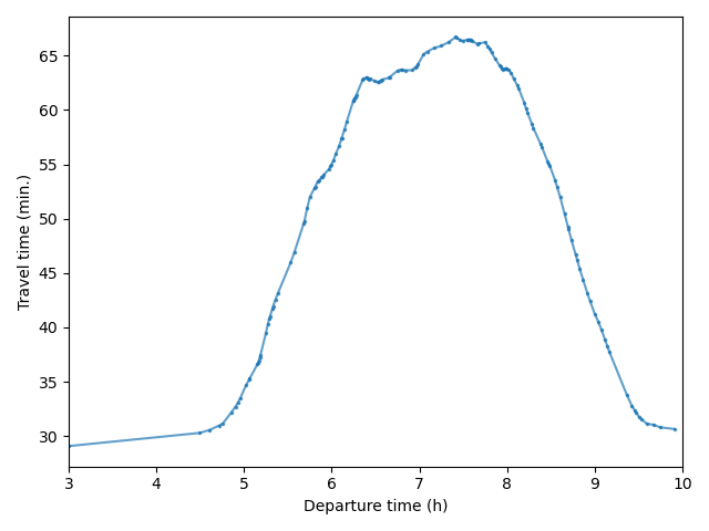
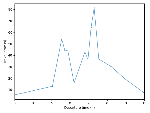
Pre-Day Model
- Input: agents' characteristics and origin-destination travel-time functions
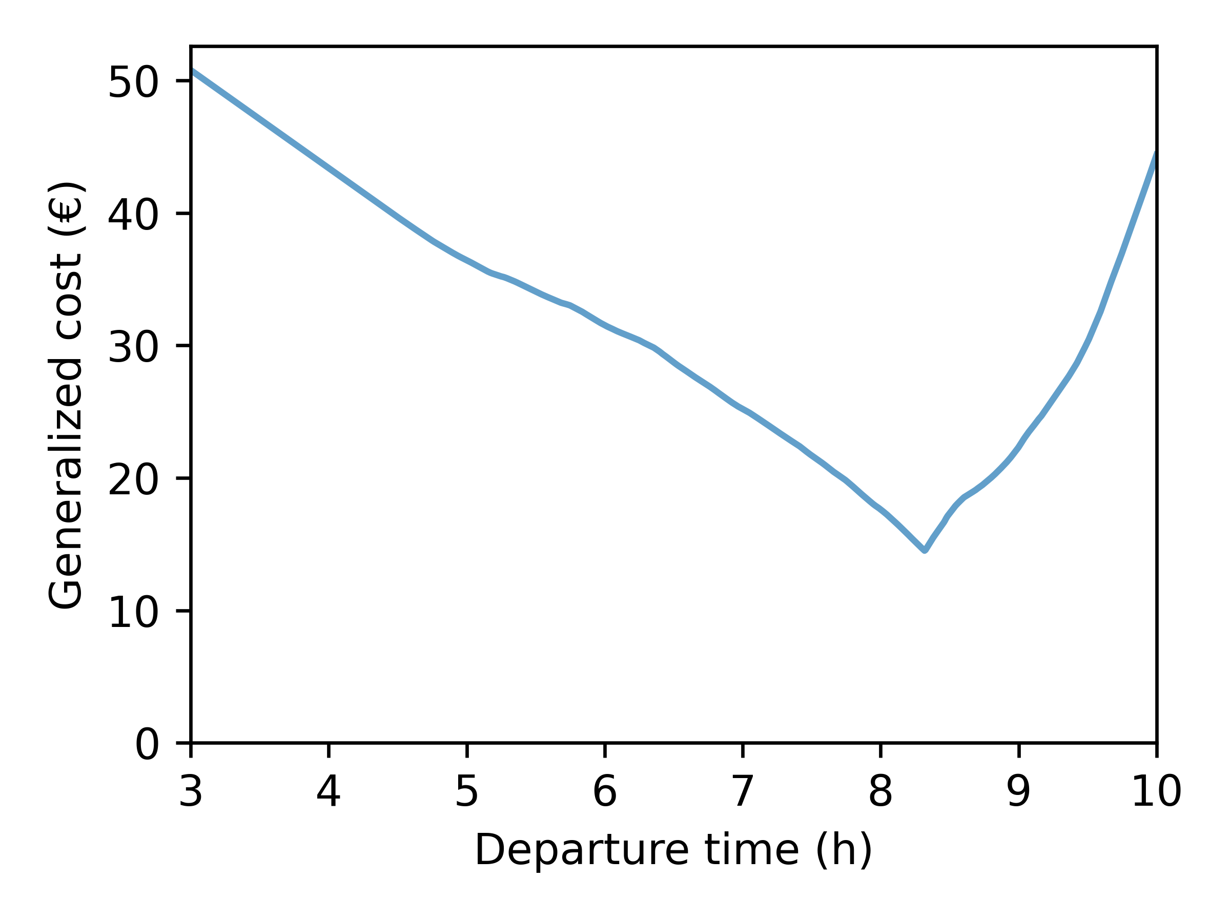
- Step 1: Compute generalized costs
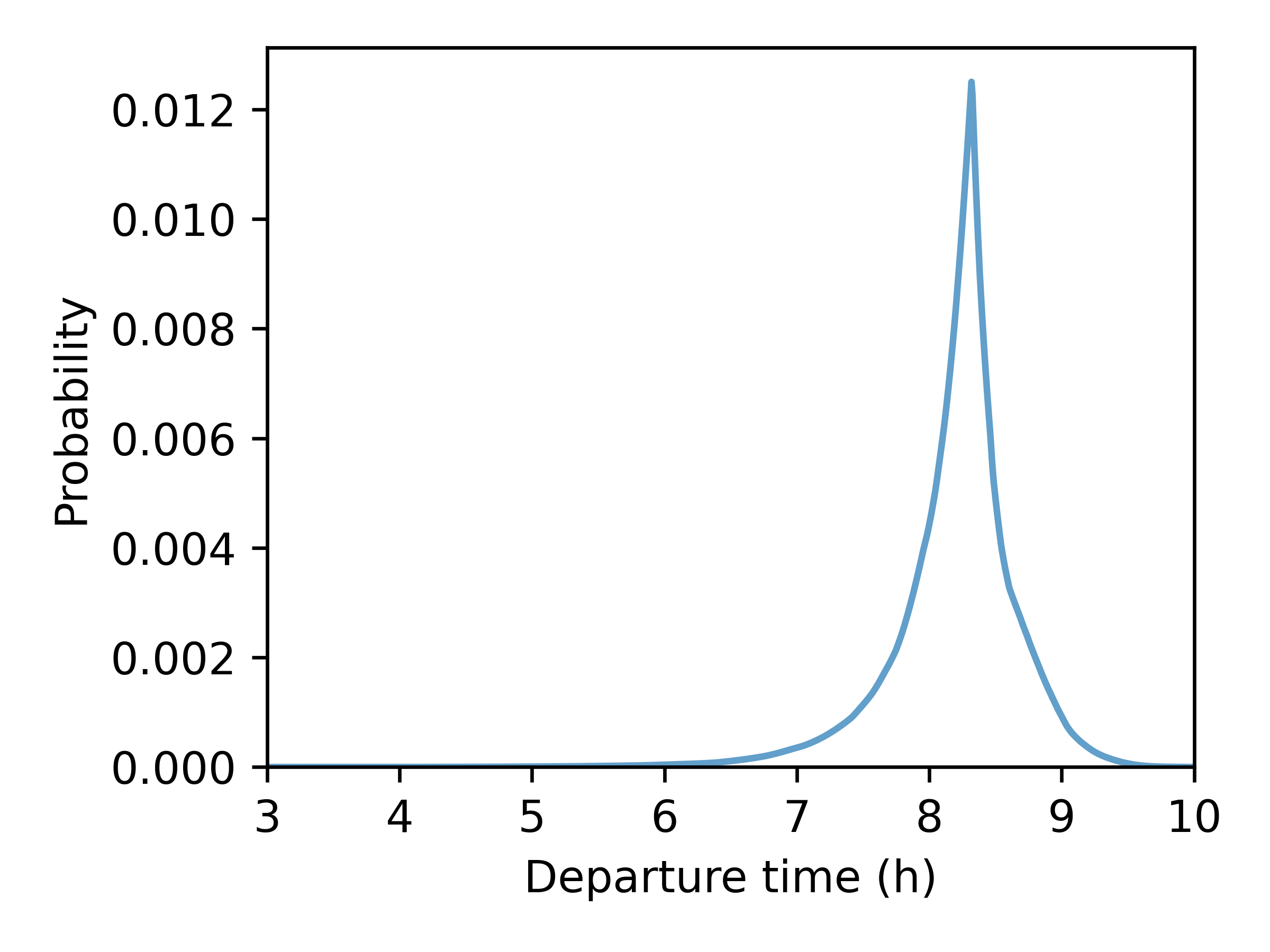
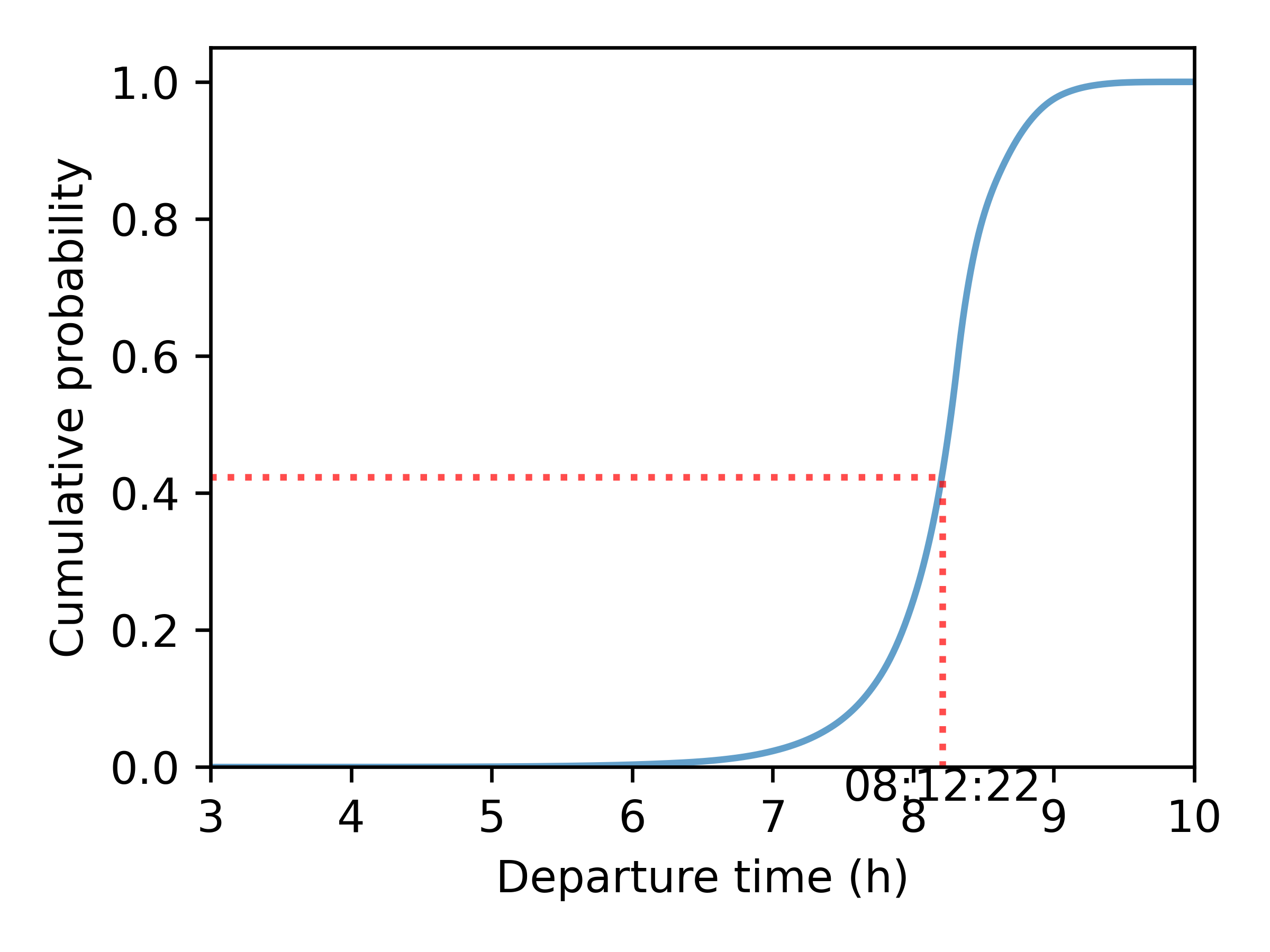
- Step 2: Find chosen departure time (Continuous Logit Model)
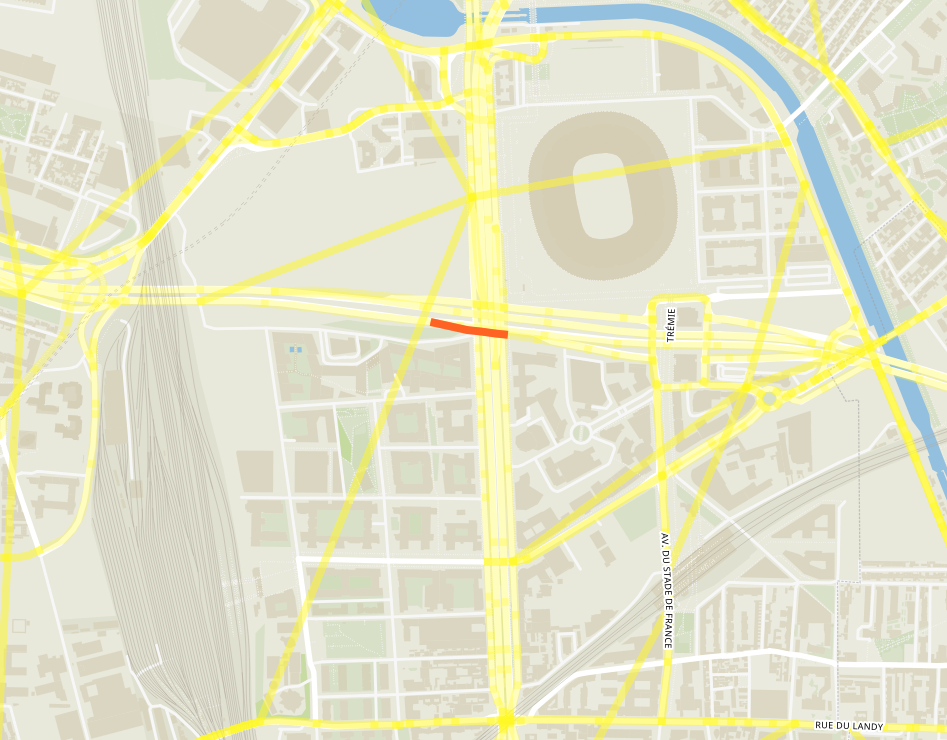
- Step 3: Find chosen route (fastest path given departure time)
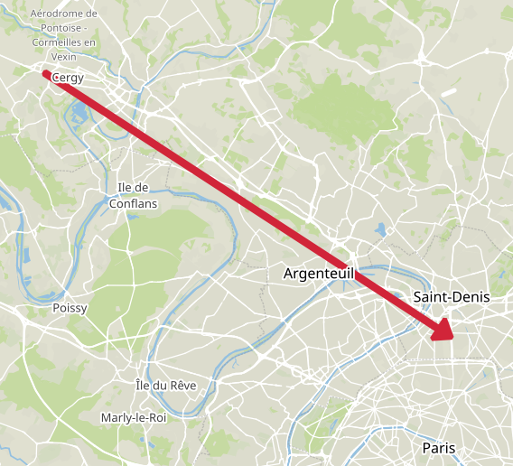
- Origin: 951270127 (Cergy – Justice-Heuruelles)
- Destination: 930661102 (Saint-Denis – Plaine 02)
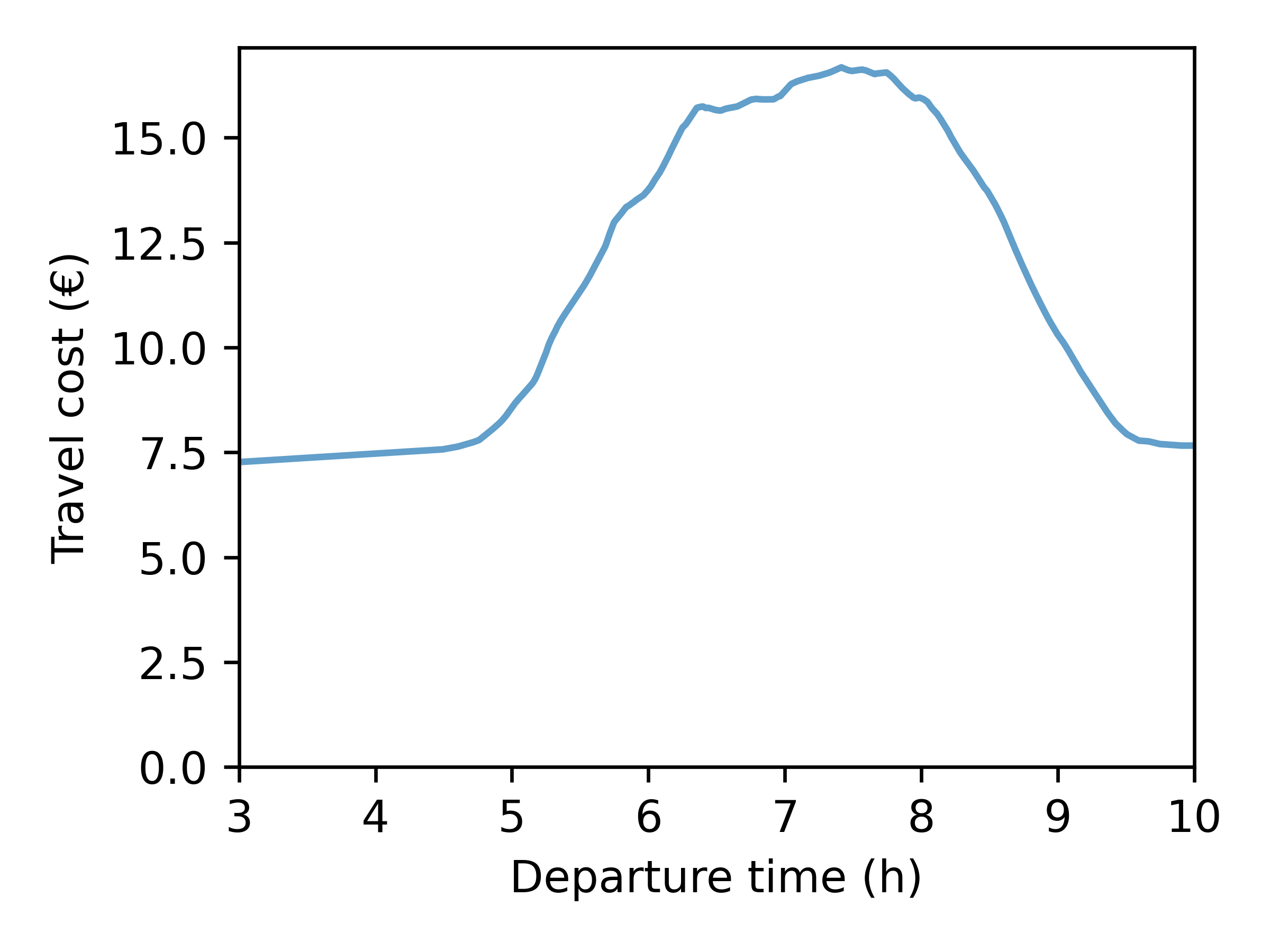
- Value of time: 15 euros / hour
- Early penalty: 7.5 euros / hour
- Late penalty: 30 euros / hour
- Desired arrival time: 09:15
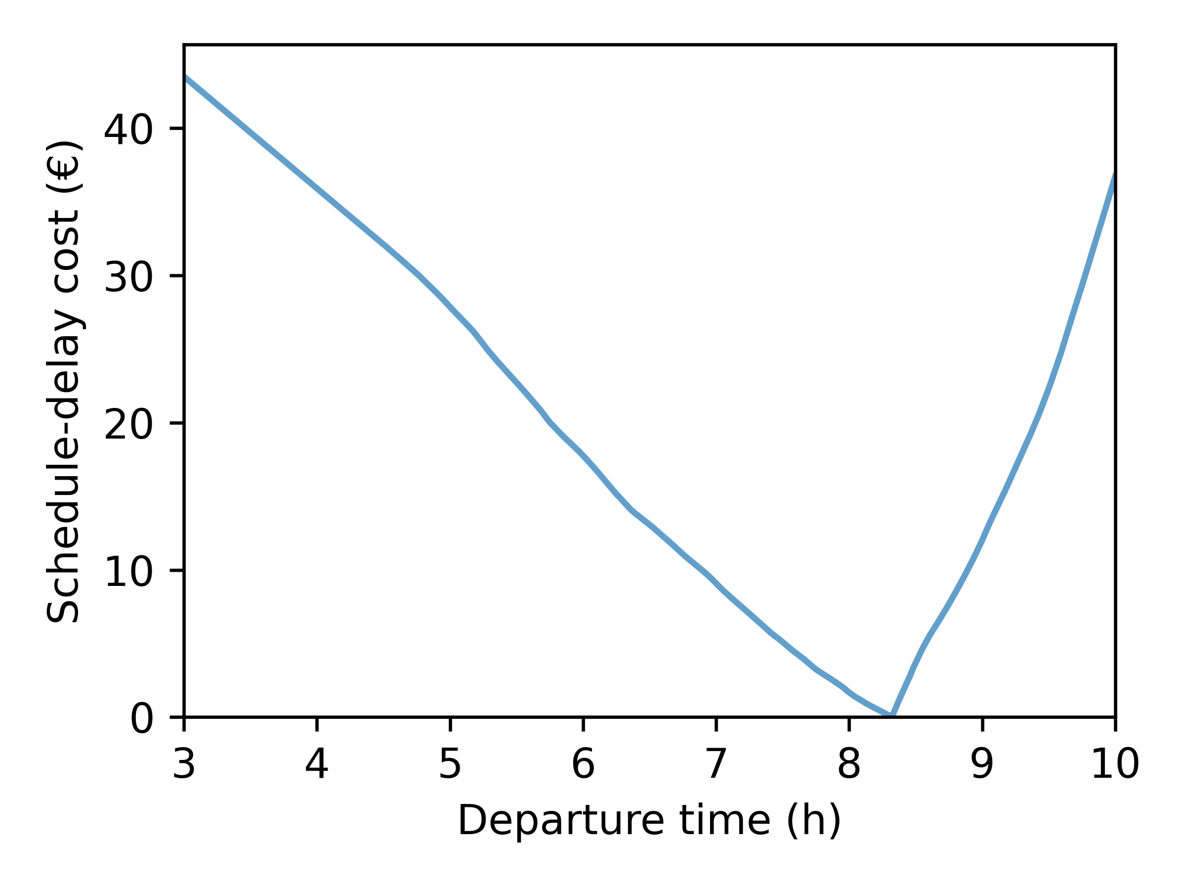
\[ c(t_d, t_a) = \underbrace{\alpha \cdot (t_a - t_d)}_{\text{travel cost}} + \underbrace{\beta \cdot [t^* - t_a]_+ + \gamma \cdot [t_a - t^*]_+}_{\text{schedule-delay cost}} \]
+
=
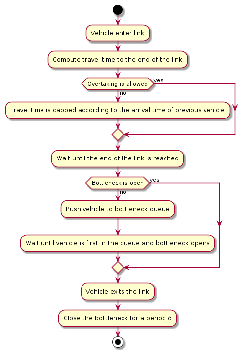
Within-Day Model
- Input: Chosen mode, departure time and route of each agent
- Agents' actions are simulated in a chronological order
- Congestion is simulated with speed-density functions and bottlenecks
- Output: Edges' travel-time functions
| Time | Event |
|---|---|
| 03:00:03 | Agent 91735 leaves origin through edge 317770 |
| 03:00:11 | Agent 111697 leaves origin through edge 161026 |
| 03:00:11 | Agent 157315 leaves origin through edge 99613 |
| 03:00:18 | Agent 134340 leaves origin through edge 68763 |
| 03:00:21 | Agent 152934 leaves origin through edge 137501 |
| 03:00:31 | Agent 43475 leaves origin through edge 16265 |
| 03:00:34 | Agent 111697 takes edge 161020 |

Day-to-Day Model
- Input: Expected and simulated edges' travel-time functions
- Learning process based on Markov decision processes
- Stop the simulation if a stopping criteria is reached (e.g., maximum number of iterations, difference between expected and simulated travel times)
- Output: Expected edges' travel-time functions for next iteration
\[ {tt}^e_{\tau + 1} = \lambda \cdot {tt}^e_{\tau} + (1 - \lambda) \cdot {tt}^s_{\tau} \]
Calibration
Travel time penalties at intersections are calibrated to match travel time distribution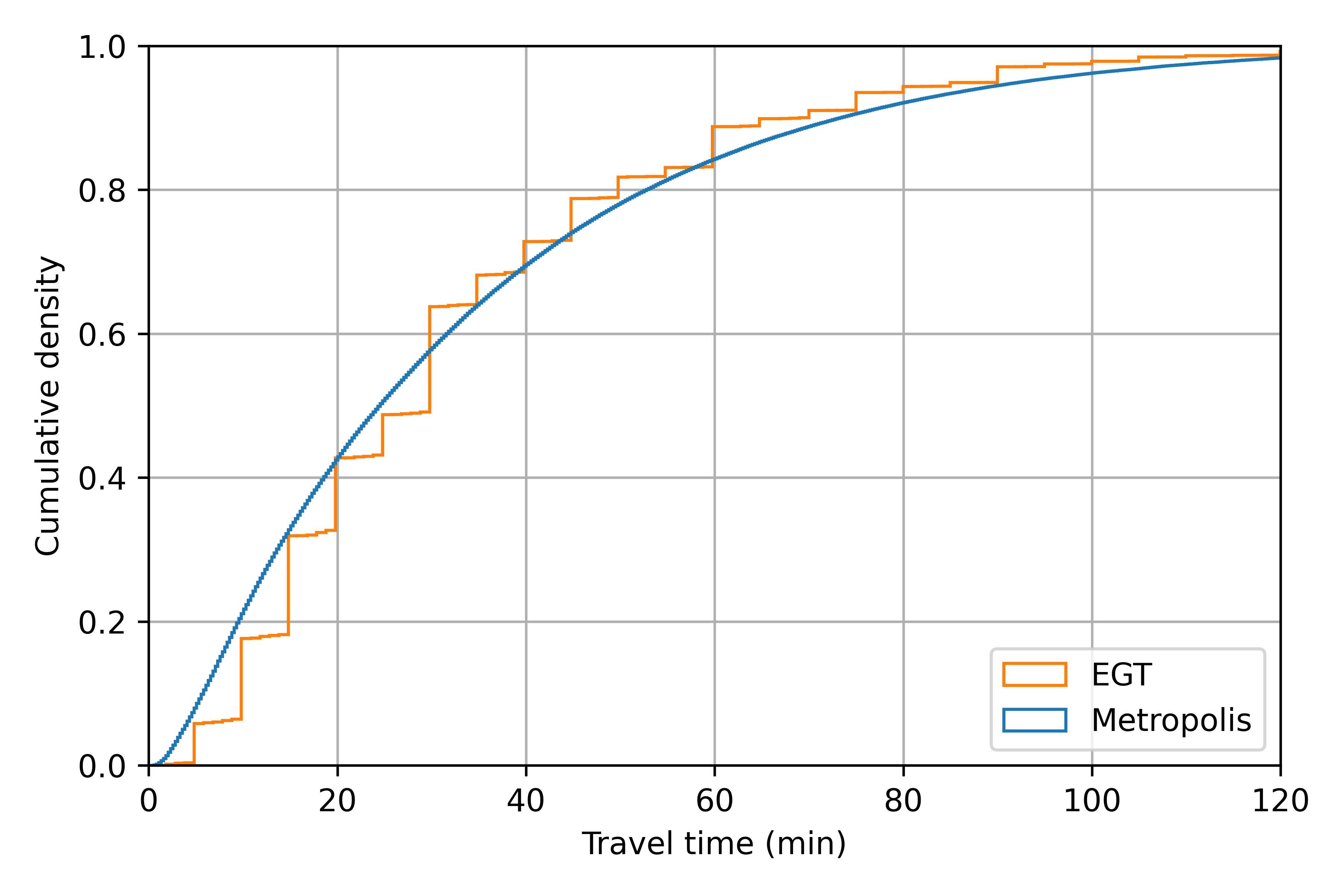
Calibration
Distribution of desired arrival times is calibrated to match arrival time distribution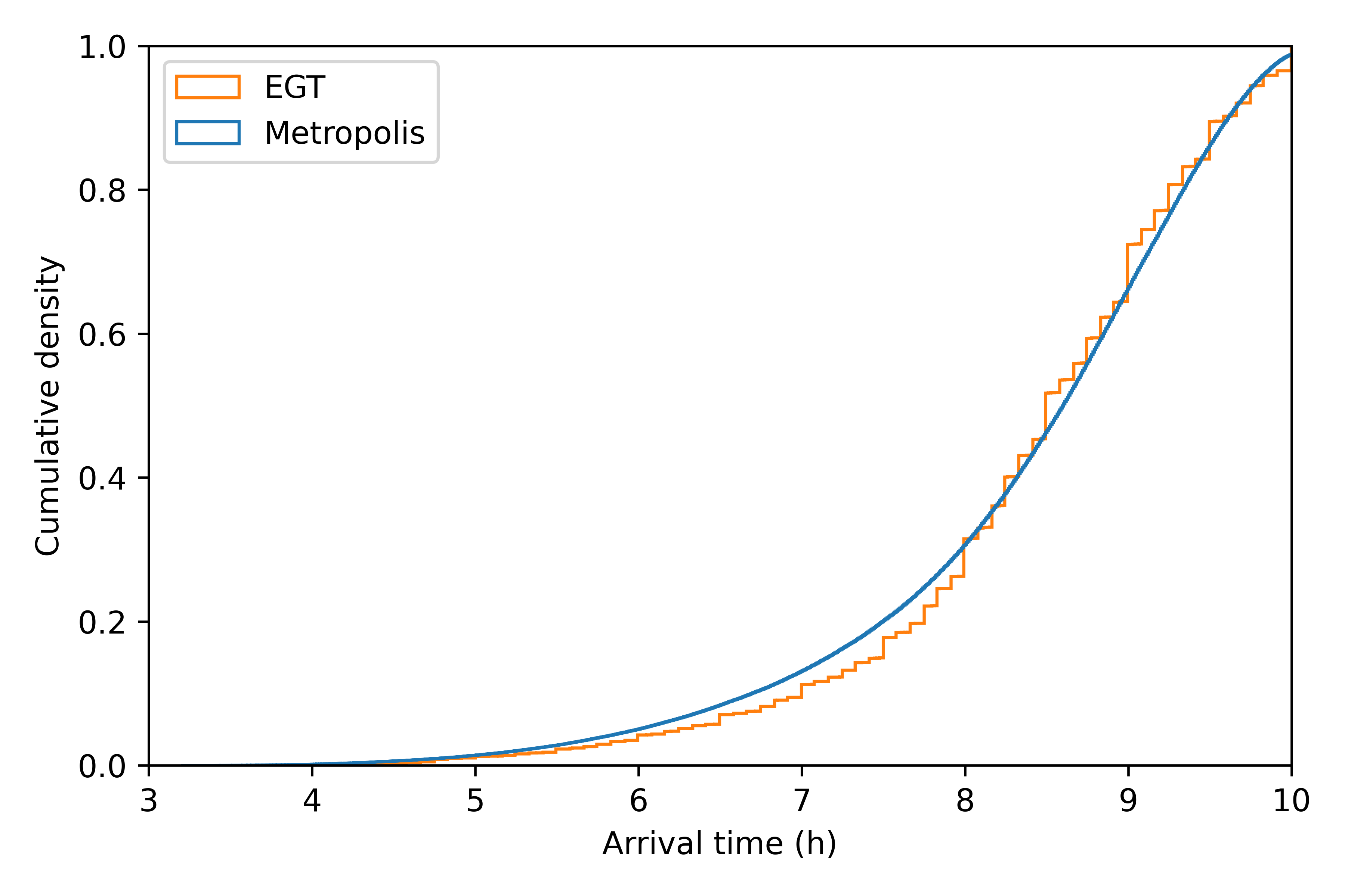
Results
Cost of congestion: 3€ TO BE COMPLETEDPolicy
What happen if we remove 20% of agents at random? TO BE COMPLETEDConclusion
Public Transit
TO BE COMPLETEDFuture improvements
- Automatic computation of air pollution
- Road maintenance
- Ride-sharing